k-armed Bandit Problem

다음 문제를 생각해 보자.

철수는 미국 여행 중 라스베가스 공항을 경유하게 되었다. 다음 비행기는 2시간 후 출발할 예정이라, 철수는 그동안 라스베가스 공항의 명물, 슬롯머신을 당겨 보기로 했다. 다행히 공항에 사람이 별로 없어서 철수는 10대의 슬롯머신을 독점적으로 사용할 수 있다. 각 슬롯머신에서 돈을 딸 확률은 기기마다 각자 다른 값으로 고정되어 있고, 한 번에 한 대의 슬롯머신만 당길 수 있다고 할 때, 철수는 어떤 전략을 취해야 가장 많은 돈을 딸 수 있을까?

이와 같이 k개의 선택 가능한 옵션(행동)이 있고, 한 옵션을 선택하면 고정된 확률 분포(stationary probability distribution)에 따라 보상(numerical reward)을 받을 수 있을 때, 특정 시간(횟수) 동안 받을 수 있는 전체 보상을 최대화하는 문제를 k-armed Bandit Problem 또는 Multi-armed Bandit Problem(MAB) 이라 한다.^[1]

만약 철수가 전체 슬롯머신의 당첨 확률 분포를 정확히 알고 있다면, 당연히 그 중 가장 높은 당첨 기댓값을 가진 기기만 2시간 내내 당기는 것이 가장 많은 돈을 따는 방법일 것이다. 하지만 철수는 ~~당연히~~ 슬롯머신들의 확률 분포를 정확히 모르기에 여러 번의 시행착오를 통해 이를 추정해야 한다. 이때 이전 글에서 살펴본 Exploitation과 Exploration 사이의 딜레마가 적용된다. k-armed Bandit Problem에서 당첨 기댓값은 가치(value)의 역할을 한다. 여러 행동들 중 현재 추정하고 있는 가치가 가장 큰 행동, 즉 현재 추정 중인 최선 행동(optimal action)을 탐욕적 행동(greedy action) 이라 한다. 만약 철수가 탐욕적 행동을 수행한다면(= 당첨 기댓값이 가장 높은 슬롯 머신을 당긴다면) 철수는 Exploitation을 수행한 것이다. 그러나 철수가 비탐욕적 행동(nongreedy action)^[2]을 수행한다면 철수는 Exploration을 수행한 것이다. 비탐욕적 행동을 수행하면 그 과정에서 확률 분포를 더 정확히 추정할 수 있게 되기 때문이다.^[3] 더 많은 Exploration을 진행할수록 더 정확한 당첨 확률 분포를 알 수 있겠지만, 전체 시간 제한이 있으므로(2시간) Exploration에 너무 많은 시간을 투자하면 Exploitation 시간이 줄어, 막상 결과적으로 얻는 최종 액수는 적어질 것이다. Exploitation과 Exploration 둘 중 어떤 것을 할지 결정하기 위해서는 추정한 가치의 정확도(precision), 불확실성(uncertainty), 남은 횟수(remaining step) 등 다양한 값들을 복합적으로 고려해야 한다.

Action-value Method

Action-value Method란 각 행동으로 인해 얻을 수 있을 가치를 추정하여, 다음 행동을 선택할 때 이를 사용하는 방법을 뜻한다.

Sample-average Method

각 행동의 가치를 추정하는 가장 간단한 방법은 Sample-average Method이다. 이 방법은 이때까지의 실험 결과로 얻은 보상들의 평균을 가치로 사용하는 방법이다. 즉 특정 시간 $t$ 에서 특정 행동 $a$ 의 가치를 $Q_{t} (a)$ 라 할 때,

Q_{t} (a) = \frac{시간 t 이전에 a 가 실행되며 받은 모든 보상의 합}{시간 t 이전에 a 가 실행된 횟수} = \frac{\sum_{i = 1}^{t - 1} R_{i} \cdot 1_{A_{i} = a}}{\sum_{i = 1}^{t - 1} 1_{A_{i} = a}}

이라 추정하는 것이다. 여기서 $1_{p r e d i c a t e}$ 는 $p r e d i c a t e$ 조건이 참일 때 1, 거짓일 때 0이 되는 확률 변수(random variable)를 뜻하고, $A_{i}$ 는 시간 $i$ ( $\leq t$ )에 시행한 행동을 뜻한다. 즉 시간 $i$ 에 행동 $a$ 를 수행했다면 $1_{A_{i} = a} = 1$ 이 되고, 시간 $i$ 에 $a$ 가 아닌 다른 행동을 수행했다면 $1_{A_{i} = a} = 0$ 이 된다. 만약 위 식에서 분모가 0이면(즉 시간 $t$ 동안 행동 $a$ 가 한 번도 시행되지 않았다면) $Q_{t} (a)$ 로 적당한 기본값(ex. 0)을 사용한다.

큰 수의 법칙(the law of large numbers)에 의해, $a$ 를 여러 번 시행하면 할 수록 $Q_{t} (a)$ 는 실제 가치 $q_{*} (a)$ 로 수렴한다.

ε-greedy Method

추정된 가치를 바탕으로 다음 행동을 선택하는 가장 간단한 방법은 $ε$ -greedy Method이다. 이 방법은 대체로(1- $ε$ 의 확률로) 탐욕적 행동을 선택하다가, 간간히( $ε$ 의 확률로) 가능한 모든 행동들 중 하나를 무작위로 선택하는 방법이다. $ε$ 의 확률로 행동을 무작위로 선택할 때는 추정한 행동들의 가치와 독립적으로, 모든 행동들이 동일한 확률을 가지고 있는 상태에서 하나를 뽑는다. 즉 $1 - ε$ 의 확률로 Exploitation을 수행하고, $ε$ 의 확률로 Exploration을 수행하는 것이다.

그렇다면 $ε$ 이 얼마일 때가 가장 좋을까? 이를 확인하기 위해서 k-armed Testbed를 사용할 수 있다. k-armed Testbed는 k-armed Bandit Problem을 해결하기 위한 Action-value Method의 성능을 비교하기 위해 사용하는 데이터 셋으로, 다음과 같은 방법으로 만든다.

$k$ 개의 행동들에 대해, 각 행동 $a_{i}$ ( $1 \leq i \leq k$ )의 가치의 참값 $q_{*} (a_{i})$ 는 평균 0, 분산 1인 정규분보에서 무작위로 추출한다.
특정 시간 $t$ 에서 특정 행동 $A_{t} \in {a_{i} ∥ 1 \leq i \leq k}$ 가 선택되었을 때, 이 행동으로 받는 보상 $R_{t}$ 는 평균 $q_{*} (A_{t})$ , 분산 1인 정규분포에서 무작위로 추출한다.

Fig.01 10-armed Testbed
출처 : Richard S. Sutton, Andrew G. Barto, , 2nd Edition, pg. 28, Figure 2.1

10-armed Testbed를 이용해 $ε = 0.001$ , $ε = 0.1$ , $ε = 0$ (Greedy Method)일 때의 $ε$ -greedy Method의 성능을 비교해 보자.

Code :

ε

-greedy Method, 10-armed Testbed

python

import numpy as np
from matplotlib import pyplot as plt

class GreedyAgent:
    def __init__(self, k, epsilon):
        self.k = k
        self.count = np.zeros(k, dtype=int)
        self.reward_sum = np.zeros(k, dtype=float)
        self.epsilon = epsilon
    
    def getEstimatedValues(self):
        return np.divide(self.reward_sum, self.count, out=np.zeros_like(self.reward_sum), where=self.count!=0)
    
    def chooseAction(self):
        if np.random.random() < self.epsilon: # exploration
            action = np.random.choice(self.k)
        else: # exploitation
            max_actions = np.argwhere(self.getEstimatedValues() == np.max(self.getEstimatedValues())).flatten()
            action = np.random.choice(max_actions)
            
        return action
    
    def train(self, action, reward):
        self.count[action] += 1
        self.reward_sum[action] += reward
        
    def getTotalReward(self):
        return np.sum(self.reward_sum)
    
    def getAverageReward(self):
        return self.getTotalReward() / np.sum(self.count)

class Testbed:
    def __init__(self, k):
        self.true_values = np.random.normal(size=k)
        self.k = k
    
    def sample(self, action):
        assert action in range(self.k), "Invalid param:action"
        return np.random.normal(loc=self.true_values[action], scale=1)
    
    def getTrueValues(self):
        return self.true_values

steps = 2000
repeats = 100
epsilons = [0, 0.1, 0.01]
k = 10

average_rewards_sum = np.zeros((len(epsilons), steps), dtype=float)
optimal_action_count = np.zeros((len(epsilons), steps), dtype=int)
for repeat in range(repeats):
    testbed = Testbed(k=k)
    agents = [GreedyAgent(k=k, epsilon=e) for e in epsilons]
    
    optimal_action = np.argmax(testbed.getTrueValues())
    
    for i, agent in enumerate(agents):
        average_rewards = np.zeros(steps, dtype=float)
        
        for step in range(steps):
            action = agent.chooseAction()
            sample = testbed.sample(action=action)
            agent.train(action=action, reward=sample)
            
            average_rewards[step] = agent.getAverageReward()
            if action == optimal_action:
                optimal_action_count[i][step] += 1
            
        average_rewards_sum[i] += average_rewards

average_rewards_sum = average_rewards_sum / repeats
optimal_action_count = optimal_action_count / repeats

for i in range(len(epsilons)):
    line = plt.plot(np.arange(steps) + 1, average_rewards_sum[i], label=f"{epsilons[i]}-greedy")
    
plt.title("Average Reward")
plt.xlabel("Steps")
plt.ylabel("Average Reward")
plt.legend()
plt.show()

for i in range(len(epsilons)):
    plt.plot(np.arange(steps) + 1, optimal_action_count[i], label=f"{epsilons[i]}-greedy")
    
plt.title("Optimal Action Rate")
plt.xlabel("Steps")
plt.ylabel("Optimal Action Rate")
plt.legend()
plt.show()

코드 설명

line 4 ~ 31 : $ε$ -greedy Method를 수행하는 에이전트
- line 5 : GreedyAgent.__init__() 메서드
  - k-armed bandit problem에서의 k(당길 수 있는 팔 수), $ε$ 값을 인자로 받음
- line 11 : GreedyAgent.getEstimatedValues() 메서드
  - Sample-average Method로 이때까지의 수행 결과로부터 가치(value)를 예상한 값을 반환
- line 14 : GreedyAgent.chooseAction() 메서드
  - 0 이상 1 미만의 랜덤값에 대해, 그 값이 $ε$ 보다 작으면(즉 $ε$ 의 확률로) 탐색(Exploration)을, $ε$ 보다 크면(즉 $1 - ε$ 의 확률로) 활용(Exploitation)을 수행
- line 23 : GreedyAgent.train() 메서드
  - 행동 action을 시행해 reward만큼의 보상을 받았을 때, 이 메서드를 이용해 이 경험을 저장한다.
- line 27, 30 : GreedyAgent.getTotalReward(), GreedyAgent.getAverageReward() 메서드
  - 각각 이때까지의 시행 동안 받은 모든 보상의 합, 평균을 반환
line 33 ~ 43 : k-armed Testbed
- line 34 : Testbed.__init__() 메서드
  - k-armed Testbed에서의 k 값을 인자로 받음
- line 38 : Testbed.sample() 메서드
  - 행동 action을 시행했을 때의 보상을 출력
- line 42 : Testbed.getTrueValues() 메서드
  - k-armed Testbed의 실제 가치(value)를 출력
line 45 ~ 48 : 각 게임당 팔을 당길 수 있는 기회 횟수 steps, 시뮬레이션을 반복할 횟수 repeats, 시도해 볼 에이전트의 종류 epsilons, 당길 수 있는 팔 수 k 초기화
line 52 ~ 73 : 총 repeats번 시뮬레이션 진행
- 한 시뮬레이션에서는 다음 과정을 진행
  - line 53 : Testbed 생성
  - line 54 : epsilons에 있는 값들을 $ε$ 으로 가지는 $ε$ -greedy 에이전트 생성
  - line 56 : 생성된 Testbed로부터 최적 행동(= 가치가 가장 큰 행동)을 찾아 저장 (Optimal Action Rate 계산할 때 사용할 예정)
  - line 58 ~ 70 : 각 에이전트마다 총 steps번 행동을 수행
line 75 ~ 82 : Average Reward 그래프 그리기
line 84 ~ 91 : Optimal Action Rate 그래프 그리기

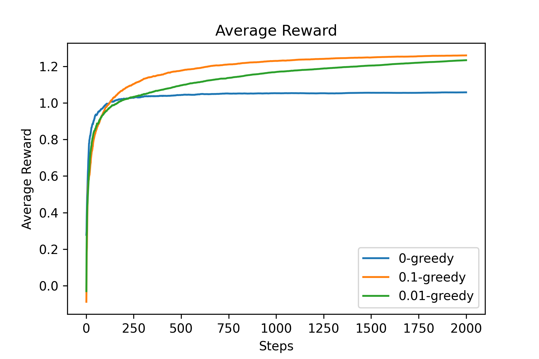
Fig.02 Average Reward (예시)
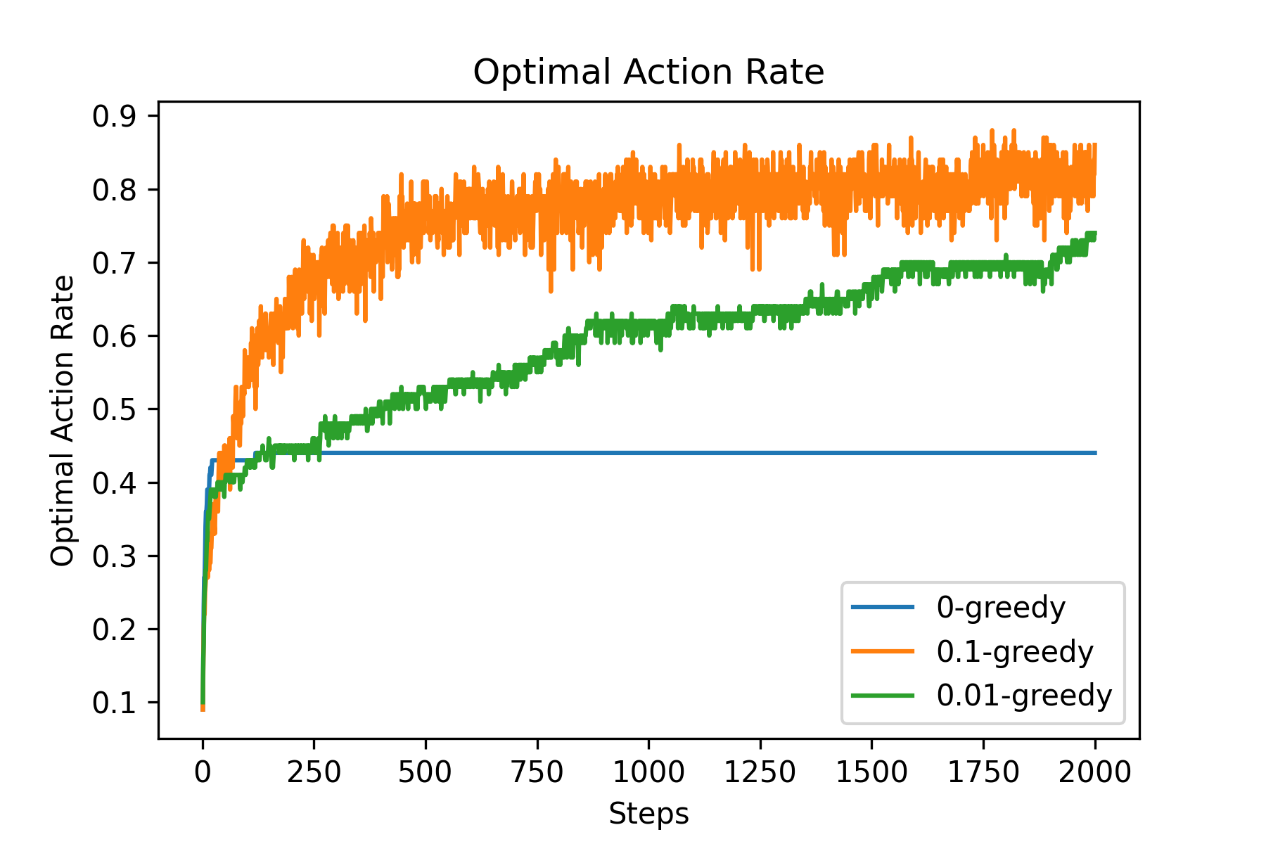
$ε = 0$ , $ε = 0.1$ , $ε = 0.01$ 으로 하여 $ε$ -greedy Method를 적용 (k=10, steps=2000, repeats=100)

Fig.03 Optimal Action Rate (예시)
$ε = 0$ , $ε = 0.1$ , $ε = 0.01$ 으로 하여 $ε$ -greedy Method를 적용 (k=10, steps=2000, repeats=100)

위 그래프에서 볼 수 있듯이 $ε$ 이 얼마든 $ε$ -greedy Method를 적용하면 경험이 쌓일수록 받을 수 있는 평균 보상이 커진다. 특히 Greedy Method( $ε = 0$ )의 경우 처음에는 다른 방법들보다 조금 더 빨리 좋아지지만, 최적 행동(optimal action)이 아닌 차(次)적 행동(suboptimal action)에 빠지기 쉬워 시간이 지나면 가장 낮은 성능을 보이게 된다. 한편 $ε = 0.01$ 일 때는 $ε = 0.1$ 일 때보다 최적 행동을 찾는데 더 오랜 시간이 걸려 비교적 천천히 좋아진다. 하지만 충분히 오랜 시간이 지나면 최적 행동을 최대 91%의 확률로만 시행할 수 있는 $ε = 0.1$ 보다 최대 99.1%의 확률로 시행할 수 있는 $ε = 0.01$ 가 받는 보상이 더 많아진다. 만약 시간이 지남에 따라 점점 감소하는 $ε$ 을 사용한다면 $ε$ 이 클 때의 장점(빠르게 최적 행동을 찾는다)과 $ε$ 이 작을 때의 장점(최적 행동을 많이 시행해 받는 보상을 최대화한다)을 합칠 수 있다.

사실 최적의 $ε$ 값은 지금 풀고자 하는 문제에 따라 달라진다. 만약 Testbed의 분산이 1이 아닌 10이라면, $ε$ 의 값이 커야 좋을 것이다. 하지만 만약 분산이 0이라면 Greedy Method( $ε = 0$ )이 가장 좋은 방법일 것이다. 또한 만약 각 행동들의 실제 가치(true value) $q_{*} (a)$ 가 고정되어 있지 않다면(nonstationary) 탐색(exploration)이 매우 중요해진다. 탐색을 통해 현재 추정 중인 최선의 행동보다 더 좋은 행동이 있는지를 찾아야 하기 때문이다.

Incremental Implementation

Sample-average Method는 각 행동의 가치를 추정한 값으로 각 행동들이 이때까지 시행 결과 받은 시행당 평균 보상을 사용한다. 이를 위해서 위 코드에서는 가치 추정값을 사용할 때마다 각 행동이 선택되어 받은 보상의 합을 저장하는 reward_sum 변수를 각 행동들이 선택된 횟수를 저장하는 count 변수로 나눠 매번 평균을 계산했다. 총 $k$ 개의 행동이 있다고 할 때, 이 방법은 매 시행마다 $k$ 번의 나눗셈 연산이 필요하다. 이를 최적화할 수는 없을까?

만약 특정 행동이 이때까지 $n - 1$ 번 뽑혔고, 그때마다 각각 $R_{1}$ , $R_{2}$ , ..., $R_{n - 1}$ 만큼의 보상을 받았다 해 보자. 그렇다면 해당 행동의 가치 $Q_{n}$ ^[4]은 다음과 같이 계산 가능하다.

Q_{n} = \frac{R_{1} + R_{2} + \dots + R_{n - 1}}{n - 1}

그렇다면 $Q_{n + 1}$ 은 다음과 같이 계산할 수 있다.

\begin{aligned} Q_{n + 1} & = \frac{R_{1} + R_{2} + \dots + R_{n}}{n} \\ = \frac{R_{1} + R_{2} + \dots + R_{n - 1}}{n - 1} \cdot \frac{n - 1}{n} + \frac{R_{n}}{n} \\ = Q_{n} \cdot (1 - \frac{1}{n}) + \frac{R_{n}}{n} \\ = Q_{n} + \frac{1}{n} (R_{n} - Q_{n}) \end{aligned}

이렇게 하면 매 시행마다 단 한 번의 나눗셈 연산이면 충분하다. 이와 같이 업데이트 식을 이전 항으로부터 연속적으로 계산할 수 있는 점화식의 형태로 구현하는 것을 Incremental Implementation이라 한다.

여담 : $Q_{n + 1} = Q_{n} + α (R_{n} - Q_{n})$

위 문단에서 살펴본 식을 조금 더 자세히 분석해보자.

Q_{n + 1} = Q_{n} + \frac{1}{n} (R_{n} - Q_{n})

사실 위 식은 강화학습에 자주 등장하는, 아주 전형적인 형태의 식이다.

(새 추정값) = (이전 추전값) + (스텝 크기) · [(목표값) - (이전 추정값)]

이 식에서 [(목표값) - (이전 추정값)] 항은 목표값과 이전 추정값 사이의 오차(error)를 구하는 항이다. 위 식을 계속 적용해 나가면 목표값과 추정값 사이의 오차는 점점 줄어들게 된다(= 추정값과 목표값은 점점 유사해진다). 식이 한 번 수행될 때마다 추정값은 (스텝 크기)만큼 목표값에 다가가게 된다. 일반적으로 스텝 크기(step size)는 $α_{t} (a)$ 또는 그냥 간단히 $α$ 라 표기한다. Sample-average Method는 스텝 크기로 $\frac{1}{n}$ 을 사용한다(= 매 시행마다 $\frac{1}{n}$ 씩 가까워진다).

Q_{n + 1} = Q_{n} + α (R_{n} - Q_{n})

Sample-average Method에서 $Q_{n}$ 이 가까워져야 할 목표값은 사실 $q_{*} (a)$ 이다. 하지만 $q_{*} (a)$ 은 알 수 없으므로 비록 약간의 노이즈(noise)가 있지만 $R_{n}$ 을 목표값으로 삼고 움직인다. $q_{*} (a)$ 의 확률 분포가 고정되어(stationary) 있다면 시행 횟수가 충분히 큰 경우 $Q_{n}$ 은 $q_{*} (a)$ 에 수렴한다.

구현

Incremental Implementation을 적용하여 위 코드의 GreedyAgent를 다시 구현하면 다음과 같이 된다.

Code :

ε

-greedy Method, Incremental Implementation

python

class GreedyAgent:
    def __init__(self, k, epsilon):
        self.k = k
        self.count = np.zeros(k, dtype=int)
        self.estimated_values = np.zeros(k, dtype=float)
        self.epsilon = epsilon
    
    def getEstimatedValues(self):
        return self.estimated_values
    
    def chooseAction(self):
        if np.random.random() < self.epsilon: # exploration
            action = np.random.choice(self.k)
        else: # exploitation
            max_actions = np.argwhere(self.getEstimatedValues() == np.max(self.getEstimatedValues())).flatten()
            action = np.random.choice(max_actions)
            
        return action
    
    def train(self, action, reward):
        self.count[action] += 1
        self.estimated_values[action] = self.estimated_values[action] + (1/self.count[action]) * (reward - self.estimated_values[action])
        
    def getTotalReward(self):
        return np.sum(self.estimated_values * self.count)
    
    def getAverageReward(self):
        return self.getTotalReward() / np.sum(self.count)

코드 설명

line 5 : 이때까지 받은 보상의 합을 저장하던 reward_sum 변수 대신, 가치 추정치를 저장하는 estimated_values 변수 사용
line 9 : 매번 GreedyAgent.getEstimatedValues() 메서드가 호출될 때마다 평균값을 계산하는 대신, 이미 계산된 estimated_values를 반환
line 22 : Incremental Implementation 적용
line 25, line 28 : estimated_values을 사용하는 방법으로 변경

Nonstationary Bandit Problem

원래 k-armed Bandit Problem에서는 행동들을 선택했을 때 받을 수 있는 보상의 확률분포가 고정되어(stationary) 있었다.^[5] 그렇다면 행동들을 선택했을 때 받을 수 있는 보상의 확률분포가 고정되어 있지 않은, Nonstationary Bandit Problem은 어떻게 풀 수 있을까?

Exponential Recency-weighted Average Method

Nonstationary Bandit Problem 상황에서는 과거에 받았던 보상보다 최근에 받았던 보상에 더 큰 가중치를 주는 것이 자연스럽다. 이를 구현하는 가장 간단한 방법은 Incremental Implementation 문단에서의 $α$ 에 (0, 1] 사이의 고정된 상수를 사용하는 것이다. 이 방법을 Exponential Recency-weighted Average Method이라 한다.

Q_{n + 1} = Q_{n} + α (R_{n} - Q_{n})

(단, $α \in (0, 1]$ 는 상수)

이 식을 풀어 쓰면 다음과 같이 된다.

\begin{aligned} Q_{n + 1} & = Q_{n} + α (R_{n} - Q_{n}) \\ = α R_{n} + (1 - α) Q_{n} \\ = α R_{n} + (1 - α) [α R_{n - 1} + (1 - α) Q_{n - 1}] \\ = α R_{n} + (1 - α) α R_{n - 1} + (1 - α)^{2} Q_{n - 1} \\ = α R_{n} + (1 - α) α R_{n - 1} + (1 - α)^{2} [α R_{n - 2} + (1 - α) Q_{n - 2}] \\ = α R_{n} + (1 - α) α R_{n - 1} + (1 - α)^{2} α R_{n - 2} + (1 - α)^{3} Q_{n - 2} \\ = ⋮ \\ = (1 - α)^{0} α R_{n} + (1 - α) α R_{n - 1} + (1 - α)^{2} α R_{n - 2} + \dots + (1 - α)^{n - 1} α R_{1} + (1 - α)^{n} Q_{1} \\ = (1 - α)^{n} Q_{1} + \sum_{i = 1}^{n} α (1 - α)^{n - i} R_{i} \end{aligned}

$α = 1$ 일 때는 $Q_{n} = R_{n}$ 이 된다.^[6] 즉, 이 경우에는 과거의 지식(경험)을 전혀 사용하지 않고, 바로 직전에 받은 보상을 가치 추청값으로 쓴다는 뜻이 된다.

이 방법을 왜 Exponential Recency-weighted Average Method이라 부를까? 우선 위 식을 잘 보면 보상들( $R_{i}$ )과 $Q_{1}$ 앞에 붙은 계수들의 합 $(1 - α)^{n} + \sum_{i = 1}^{n} α (1 - α)^{n - i}$ 은 항상 1임을 알 수 있다. 즉 이 식은 가중 평균(Weighted Average)을 구하는 식이다.

증명 :

(1 - α)^{n} + \sum_{i = 1}^{n} α (1 - α)^{n - i}

= 1

$β = 1 - α$ 라 하면 $(1 - α)^{n} + \sum_{i = 1}^{n} α (1 - α)^{n - i}$ 은 다음과 같이 된다.

\begin{aligned} (1 - α)^{n} + \sum_{i = 1}^{n} α (1 - α)^{n - i} & = (1 - α)^{n} + α [1 + (1 - α) + (1 - α)^{2} + \dots + (1 - α)^{n - 1}] \\ = β^{n} + (1 - β) (1 + β + β^{2} + \dots + β^{n - 1}) \\ = β^{n} - (β - 1) (β^{n - 1} + \dots + β^{2} + β + 1) \\ = β^{n} - (β^{n} - 1) \\ = 1 \end{aligned}

또한 각 보상 $R_{i}$ 에 붙는 가중치 $α (1 - α)^{n - i}$ 는 $n - i$ 에 영향을 받는다. $0 \leq n - i < 1$ 이므로, 더 오래된 보상일수록(= $i$ 가 작을수록 = 가장 최근 보상과 해당 보상 사이에 받은 보상의 개수 $n - i$ 가 많을수록) 가중치는 기하급수적으로 작아지고, 반대로 최근에 받은 보상일수록 가중치가 기하급수적으로 커진다. 이 때문에 $α$ 에 상수를 쓰는 이 방법을 Exponential Recency-weighted Average Method라 부르는 것이다.

여담 : $Q_{n + 1} = Q_{n} + α (R_{n} - Q_{n})$ 가 수렴할 $α$ 의 조건

위 Incremental Implementation 문단에서 유도한 식을 다시 한 번 살펴보자.

Q_{n + 1} = Q_{n} + α (R_{n} - Q_{n})

우리는 이때까지 $α$ 로 $\frac{1}{n}$ 이 사용된 경우(Sample-average Method)와, 상수가 사용된 경우(Exponential Recency-weighted Average Method), 이렇게 두 가지 경우를 보았다. $α = \frac{1}{n}$ 인 경우 큰 수의 법칙에 의해 $Q_{n}$ 은 $q_{*} (a)$ 로 수렴하지만, 상수인 경우엔 수렴하지 않는다.^[7] 이 둘 이외에도 다양한 값 또는 함수를 $α$ 로 사용할 수 있다. 그렇다면 한 가지 의문이 생긴다. 위 식을 수렴하게 하는 $α$ 의 조건은 무엇일까?

Stochastic Approximation Theory에 의하면, $α_{n} (a)$ 은 다음 조건일 때 100% 확률로 수렴한다.

\sum_{n = 1}^{\infty} α_{n} (a) = \infty and \sum_{n = 1}^{\infty} α_{n}^{2} (a) = c

(단, $c$ 는 상수)

첫 번째 조건의 의미는 $α_{n} (a)$ 가 충분히 커, 초기값이 어떻든, 노이즈가 있어도 결국 이들을 극복할 수 있다는 뜻이다. 두 번째 조건의 의미는 $α_{n} (a)$ 의 값이 충분히 작아져, 결국 수렴하게 된다는 뜻이다.

$α_{n} (a) = \frac{1}{n}$ 일 때는(Sample-average Method) 위 두 조건을 만족시키므로 수렴한다.^[8] 하지만 $α_{n} (a) = α$ 일 땐(Exponential Recency-weighted Average Method) 두 번째 조건이 성립하지 않으므로 수렴하지 않는다.

한 가지 알아두어야 할 것은 많은 경우 위 두 조건이 만족되어도 수렴 속도가 너무 느릴 수 있다는 점이다. 이런 경우 수렴이 잘 되게 하려면 상당한 튜닝이 필요하다. 그래서 위 두 조건은 이론적인 연구에서는 자주 사용되지만, 실제 응용 분야에서는 잘 사용되지 않는다.

Optimistic Initial Values

위 Incremental Implementation 문단에서 유도한 식을 다시 한 번 살펴보자.

\begin{aligned} Q_{n + 1} & = Q_{n} + α (R_{n} - Q_{n}) \\ = (1 - α)^{n} Q_{1} + \sum_{i = 1}^{n} α (1 - α)^{n - i} R_{i} \end{aligned}

$Q_{n}$ 을 구하는 식에 각 행동에 대한 초기 가치 추정값 $Q_{1}$ 이 있는 것을 볼 수 있다. $Q_{1}$ 은 일종의 편향(bias)으로서 동작하게 된다. Sample-average Method에서는 모든 행동들이 한 번씩 시행되면 편향이 없어지게 된다. 하지만 Exponential Recency-weighted Average Method에서는 편향이 없어지지 않고 계속 남아있다.

사실 이 편향은 나쁜 것이 아니다. 이를 적절히 잘 활용하면 더 효율적인 학습이 가능하게 만들 수 있다. 예를 들어 만약 우리가 각 행동들이 줄 보상에 대한 사전지식(prior knowledge)이 있다면 이를 $Q_{1}$ 에 담을 수 있다. 또한 Optimistic Initial Values라는 기법을 이용하면 탐색(Exploration)이 더 잘 일어나게 만들 수 있다.

위에서 나온 10-armed Testbed 상황을 생각해보자. 기존에는 이 Testbed에 대해 초기 가치 추정값으로 0을 사용했다. 하지만 만약 초기 가치 추정값으로 "+5"를 사용하면 어떻게 될까? 이 Testbed의 각 행동들의 실제 가치 $q_{*} (a)$ 는 평균 0, 분산 1의 정규분포를 따르므로, "+5"라는 값은 엄청나게 낙관적인(optimistic) 추정값이다. 이 상태에서 를 적용해 보자. 각 행동의 시행 결과 받는 보상은 거의 대부분의 경우 "+5"보다 작은, 아주 "실망스러운" 값일 것이다. 그 결과 에이전트는 Greedy Method( $ε = 0$ 인 $ε$ -greedy Method)를 따른다 해도 계속해서 탐색을 수행하게 된다. 이처럼 초기값으로 낙관적인 값을 줘 탐색이 더 많이 일어나게 하는 기법을 Optimistic Initial Values이라 한다.^[9]

Code :

ε

-greedy Method, Optimistic Initial Values

python

import numpy as np
from matplotlib import pyplot as plt

class GreedyAgent:
    def __init__(self, k, epsilon, q1):
        self.k = k
        self.count = np.zeros(k, dtype=int)
        self.estimated_values = np.full(shape=k, fill_value=q1, dtype=float)
        self.epsilon = epsilon
    
    def getEstimatedValues(self):
        return self.estimated_values
    
    def chooseAction(self):
        if np.random.random() < self.epsilon: # exploration
            action = np.random.choice(self.k)
        else: # exploitation
            max_actions = np.argwhere(self.getEstimatedValues() == np.max(self.getEstimatedValues())).flatten()
            action = np.random.choice(max_actions)
            
        return action
    
    def train(self, action, reward):
        self.count[action] += 1
        self.estimated_values[action] = self.estimated_values[action] + 0.1 * (reward - self.estimated_values[action])
        
    def getTotalReward(self):
        return np.sum(self.estimated_values * self.count)
    
    def getAverageReward(self):
        return self.getTotalReward() / np.sum(self.count)

class Testbed:
    def __init__(self, k):
        self.true_values = np.random.normal(size=k)
        self.k = k
    
    def sample(self, action):
        assert action in range(self.k), "Invalid param:action"
        return np.random.normal(loc=self.true_values[action], scale=1)
    
    def getTrueValues(self):
        return self.true_values

steps = 1000
repeats = 100
k = 10
configs = [{
    "epsilon": 0,
    "q1": 5
}, {
    "epsilon": 0.1,
    "q1": 0
}]

optimal_action_count = np.zeros((len(configs), steps), dtype=int)
for repeat in range(repeats):
    testbed = Testbed(k=k)
    agents = [GreedyAgent(k=k, epsilon=c["epsilon"], q1=c["q1"]) for c in configs]
    
    optimal_action = np.argmax(testbed.getTrueValues())
    
    for i, agent in enumerate(agents):        
        for step in range(steps):
            action = agent.chooseAction()
            sample = testbed.sample(action=action)
            agent.train(action=action, reward=sample)
            
            if action == optimal_action:
                optimal_action_count[i][step] += 1

optimal_action_count = optimal_action_count / repeats

for i in range(len(configs)):
    plt.plot(np.arange(steps) + 1, optimal_action_count[i], label=f"ε={configs[i]['epsilon']}, q1={configs[i]['q1']}")
    
plt.title("Optimal Action Rate")
plt.xlabel("Steps")
plt.ylabel("Optimal Action Rate")
plt.legend()
plt.show()

코드 설명

line 5 : $Q_{1}$ 을 의미하는 변수 q1을 받을 수 있게 변경
- line 8 : q1으로 초기화된 estimated_values 변수 생성
line 25 : $α = 0.1$ 로 고정
line 48 ~ 54 : $ε = 0$ , $Q_{1} = 5$ 일 때와 $ε = 0.1$ , $Q_{1} = 0$ 일 때, 이렇게 두 가지 설정값을 준비
line 59 : configs 변수에 저장된 설정값에 따라 에이전트 생성

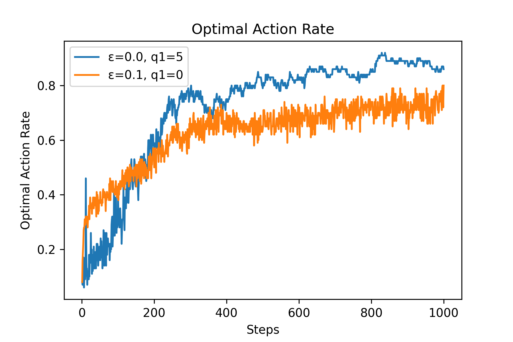
Fig.04 Optimal Action Rate (예시)
[ $ε = 0$ , $Q_{1} = 5$ ], [ $ε = 0.1$ , $Q_{1} = 0$ ]으로 하여 $ε$ -greedy Method를 적용 (k=10, steps=1000, repeats=100, $α = 0.1$ )

Fig.04에서 볼 수 있듯이 실제로 Optimistic Initial Values( $ε = 0$ , $Q_{1} = 5$ )를 사용한 경우 단순한 $ε$ -greedy Method( $ε = 0.1$ , $Q_{1} = 0$ )를 사용했을 때보다 초기에는 탐색을 많이 해 성능이 낮으나, 결국엔 성능이 더 좋아지는 것을 볼 수 있다.

그러나 Optimistic Initial Values 기법은 Stationary Problem을 풀 때는 꽤 효과적이지만, Nonstationary Problem을 풀 때는 그닥 효과적이지 않다는 단점이 있다.^[10]

UCB(Upper-Confidence-Bound) Action Selection

k-armed Bandit Problem을 풂에 있어, 탐색(Exploration)은 매우 중요하다. 탐색을 하면 행동에 대한 가치 추정값이 조금 더 정확해지기 때문이다. $ε$ -greedy Method이 Greedy Method에 비해 더 성능이 좋은 것도 탐색을 많이 하기 때문이다. 하지만 $ε$ -greedy Method은 완전 무작위로 탐색을 수행한다. 이를 조금 더 효율적으로 할 수는 없을까?

탐색을 할 때 "최적 행동이 될 가능성이 있는" 행동들만 뽑아 그 안에서 탐색을 한다면 어떨까? 이렇게 하면 조금 더 효율적인 탐색이 가능할 것이다. 그렇다면 어떤 행동이 "최적 행동이 될 가능성이 있는 행동"일까?

만약 어떤 행동이 다른 행동들보다 가치 추정값이 크다면 해당 행동이 최적 행동이 될 가능성이 높다.
만약 어떤 행동이 다른 행동들에 비해 덜 시행되어 아직 불분명하다면(베일에 쌓여 있다면) 최적 행동이 될 가능성이 높다(= 여러 번 시행해 가치 추정값이 꽤 정확해진, 가치 추정값이 낮은 행동은 최적 행동이 될 가능성이 낮다).

UCB(Upper-Confidence-Bound) Action Selection은 바로 이 점에 착안하여 만들어진 기법이다. 시간 $t$ 까지 특정 행동 $a$ 가 시행된 횟수를 $N_{t} (a)$ 라 할 때, UCB Action Selection은 다음 규칙을 이용해 행동을 선택한다.

만약 한 번도 시행되지 않은 행동이 있다면( $N_{t} (a) = 0$ ) 해당 행동을 선택한다.
만약 모든 행동들이 한 번 이상 시행되었다면 다음 식을 이용해 행동을 선택한다 :

A_{t} = \underset{a}{\arg \max} [Q_{t} (a) + c \sqrt{\frac{\ln t}{N_{t} (a)}}]

(단, $c > 0$ )

위 식의 의미를 생각해보자. 앞에서 배웠던 Greedy Method는 가장 큰 가치 추정값을 가지는 행동을 선택했다. 이를 식으로 표현하면 다음과 같이 된다.

A_{t} = \underset{a}{\arg \max} [Q_{t} (a)]

UCB Action Selection의 식은 Greedy Method의 식에 $c \sqrt{\frac{\ln t}{N_{t} (a)}}$ 항을 추가한 것이다. 이 항을 불확실도 항(uncertainty term)이라 부른다. 행동 $a$ 의 가치 추정값의 불확실도(uncertainty)를 나타내기 때문이다.

행동 $a$ 를 기준으로, $a$ 가 많이 선택될수록(= 불확실도가 내려갈수록) 분모( $N_{t} (a)$ )의 값이 커지므로 불확실도 항의 값은 작아진다. 또한 만약 다른 행동을 많이 선택했다면 분자( $\ln t$ )가 커지므로 불확실도 항의 값은 작아진다. 분자에 자연로그를 사용함으로서 시간이 지남에 따라 불확실도 항은 계속 커지지만(= unbounded) 그 증가폭은 점점 감소한다.

불확실도 항의 $c$ 는 탐색(Exploration)의 강도를 조절하는 값이다. 이 값이 크다면 더 많은 탐색을 수행하게 되고, 이 값이 작다면 더 많은 활용(Exploitation)^[11]을 수행하게 된다.

사실 Upper-Confidence-Bound란 통계학에서 신뢰구간(Confidence Interval)의 오른쪽 끝을 의미하는 말이다. 예를 들어 "정확도 95 ± 3% 테스트"에서 95 + 3 = 98%가 Upper-Confidence-Bound이다. UCB Action Selection의 이름은 바로 여기에서 나왔다. 우리의 목표는 가장 가치가 높은 행동을 뽑는 것이다. 이미 여러 번 시행된 행동의 경우 가치 추정값이 꽤 명확할 것이다. 즉 분산(variance)이 작다. 하지만 아직 몇 번 시행되지 않은 행동의 경우 가치 추정값이 불분명할 것이다. 즉 분산이 크다. 이때 UCB Action Selection은 모든 행동들에게서 동일한 면적(신뢰도)의 신뢰구간을 그린 후, 그 끝(UCB)이 가장 큰 행동을 선택하는 것이다. UCB Action Selection으로 어떤 행동이 선택되었다면, 그 행동은 가치 추정값(= 평균이 커)이 커서 선택되었을 수도 있고, 실제 가치는 작더라도 불확실성이 커(= 분산이 커) 선택되었을 수도 있다(동일한 신뢰도를 사용하기에 분산이 크면 평균(가치 추정값)이 작더라도 UCB가 커진다). 이때 신뢰도를 의미하는 파라미터가 $c$ 이다. 신뢰도가 높을수록 더 넓은 신뢰구간이 형성된다. 즉 분산이 큰(= 아직 불명확한) 행동들에 더 민감히 반응하겠다는(= 더 많이 뽑겠다는 = 탐색을 더 적극적으로 수행하겠다는) 의미가 된다.

Code : UCB Action Selection

python

import numpy as np
from matplotlib import pyplot as plt
from abc import *

class Agent(metaclass=ABCMeta):
    def __init__(self, k, q1):
        self.k = k
        self.q1 = q1
        self.estimated_values = np.full(shape=k, fill_value=q1, dtype=float)
        self.count = np.zeros(k, dtype=int)
        
    def getEstimatedValues(self):
        return self.estimated_values
    
    def reset(self):
        self.estimated_values = np.full(shape=self.k, fill_value=self.q1, dtype=float)
        self.count = np.zeros(self.k, dtype=int)
    
    @abstractmethod
    def train(self, action, reward):
        pass
    
    @abstractmethod
    def chooseAction(self, t):
        pass
    
    def getTotalReward(self):
        return np.sum(self.estimated_values * self.count)
    
    def getAverageReward(self):
        return self.getTotalReward() / np.sum(self.count)
    
    @abstractmethod
    def getName(self):
        pass

class GreedyAgent(Agent):
    def __init__(self, k, q1, epsilon):
        Agent.__init__(self, k, q1)
        self.epsilon = epsilon
    
    def chooseAction(self, t):
        if np.random.random() < self.epsilon: # exploration
            action = np.random.choice(self.k)
        else: # exploitation
            max_actions = np.argwhere(self.getEstimatedValues() == np.max(self.getEstimatedValues())).flatten()
            action = np.random.choice(max_actions)
            
        return action
    
    def train(self, action, reward):
        self.count[action] += 1
        self.estimated_values[action] = self.estimated_values[action] + (1/self.count[action]) * (reward - self.estimated_values[action])
        
    def getName(self):
        return f"ε-greedy agent [k={self.k}, q1={self.q1}, ε={self.epsilon}]"

class UCBAgent(Agent):
    def __init__(self, k, q1, c):
        Agent.__init__(self, k, q1)
        self.c = c
    
    def chooseAction(self, t):
        never_tried_actions = np.where(self.count == 0)[0]
        
        if len(never_tried_actions) != 0:
            return np.random.choice(never_tried_actions)
        
        ucb = self.estimated_values + self.c * np.sqrt((np.log(t))/(self.count))
        max_actions = np.argwhere(ucb == np.max(ucb)).flatten()
        return np.random.choice(max_actions)
    
    def train(self, action, reward):
        self.count[action] += 1
        self.estimated_values[action] = self.estimated_values[action] + (1/self.count[action]) * (reward - self.estimated_values[action])
    
    def getName(self):
        return f"ucb agent [k={self.k}, q1={self.q1}, c={self.c}]"

class Testbed:
    def __init__(self, k):
        self.true_values = np.random.normal(size=k)
        self.k = k
    
    def sample(self, action):
        assert action in range(self.k), "Invalid param:action"
        return np.random.normal(loc=self.true_values[action], scale=1)
    
    def getTrueValues(self):
        return self.true_values

steps = 1000
repeats = 100
k = 10
agents = [GreedyAgent(k=k, q1=0, epsilon=0.1), UCBAgent(k=k, q1=0, c=2)]

average_rewards_sum = np.zeros((len(agents), steps), dtype=float)
for repeat in range(repeats):
    testbed = Testbed(k=k)
    
    for i, agent in enumerate(agents):
        agent.reset()
        average_rewards = np.zeros(steps, dtype=float)
        for step in range(steps):
            action = agent.chooseAction(t=step)
            sample = testbed.sample(action=action)
            agent.train(action=action, reward=sample)
            
            average_rewards[step] = agent.getAverageReward()
        
        average_rewards_sum[i] += average_rewards

average_rewards_sum = average_rewards_sum / repeats

for i in range(len(agents)):
    line = plt.plot(np.arange(steps) + 1, average_rewards_sum[i], label=agents[i].getName())
    
plt.title("Average Reward")
plt.xlabel("Steps")
plt.ylabel("Average Reward")
plt.legend()
plt.show()

코드 설명

line 5 ~ 35 : 추상 클래스 Agent 생성
line 37 ~ 56 : Agent를 상속받은, $ε$ -greedy Method를 사용하는 에이전트
line 58 ~ 78 : Agent를 상속받은, UCB Action Selection을 사용하는 에이전트
line 80 ~ 90 : k-armed Testbed
line 92 ~ 94 : 시뮬레이션을 위한 변수값 초기화
line 95 : 에이전트 생성
line 97 ~ 113 : 시뮬레이션
line 115 ~ 122 : 그래프 출력

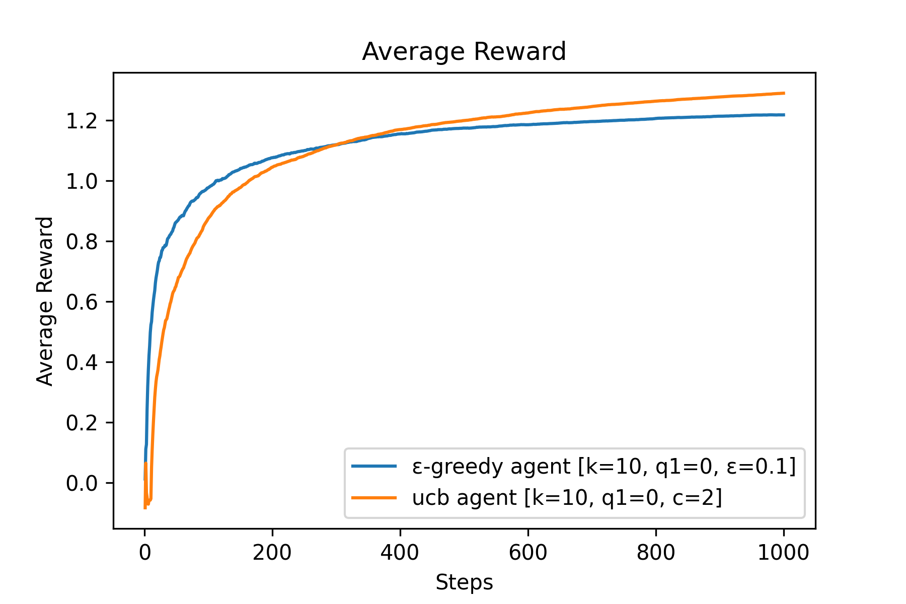
Fig.05 Average Reward (예시)
UCB Action Selection( $c = 2$ )를 사용한 에이전트와 $ε$ -greedy Method( $ε = 0.1$ )를 사용한 에이전트들의 매 단계별 평균 수령 보상 (k=10, steps=1000, repeats=100)

위 그래프에서 볼 수 있다시피 UCB Action Selection은 성능이 꽤 좋다. 하지만 이 방법에는 한계가 많다. 대표적으로 이 방법은 Nonstationary Problem에는 적용하기 힘들다. 또한 탐색해야 하는 상태 공간(state space)이 너무 크다면, 특히 함수 추정(Function Approximation)을 써야 할 정도로 상태 공간이 크다면 UCB Action Selection을 적용하기 힘들다.

Gradient Bandit Algorithm

Gradient Bandit Algorithm은 각 행동에 대한 선호도(preference)를 학습하고, 이를 기반으로 다음 행동을 선택하는 알고리즘이다. 이 알고리즘은 다음과 같이 동작한다.

시점 $t$ 에서의 행동 $a$ 의 선호도를 $H_{t} (a)$ 라 할 때, 모든 행동들의 초기 선호도 $H_{1} (a)$ 를 0으로 초기화한다.
시점 $t$ 에서 행동 $a$ 를 시행할 확률을 $π_{t} (a)$ 라 할 때, Softmax distribution(= Gibbs distribution = Boltzmann distribution)을 이용해 $π_{t} (a)$ 를 계산한 후 이를 이용해 다음 행동을 선택한다.
$π_{t} (a) = \frac{e^{H_{t} (a)}}{\sum_{b = 1}^{k} e^{H_{t} (b)}}$
$A_{t}$ 가 선택되어 시행되고 그 결과 보상 $R_{t}$ 를 받았다고 하자. 시점 $t - 1$ 까지 받은 모든 보상의 평균을 ${\bar{R}}_{t}$ 이라 할 때,^[12] Stochastic Gradient Ascent를 이용해 선호도를 업데이트한다.
${\begin{cases} H_{t + 1} (a) = H_{t} (a) + α (R_{t} - {\bar{R}}_{t}) (1 - π_{t} (a)) & (if a = A_{t}) \\ H_{t + 1} (a) = H_{t} (a) - α (R_{t} - {\bar{R}}_{t}) π_{t} (a) & (if a \neq A_{t}) \end{cases}$

이때까지의 방법들은 모두 각 행동들의 수행 결과 받은 보상을 기준으로 해당 행동의 가치(앞으로 받을 것으로 예상되는 보상)를 추정하고, 이를 기반으로 다음 행동을 선택하는 Action-value Method였다. 하지만 Gradient Bandit Algorithm은 Action-value Method가 아니다. Gradient Bandit Algorithm의 선호도는 말 그대로 해당 행동을 다른 행동에 비해 얼마나 선호하는지를 나타내는 값으로서 보상과 아무런 관계가 없다. 선호도가 크면 해당 행동은 더 자주 선택되고, 선호도가 낮으면 해당 행동은 덜 선택된다. 단적으로, 각 행동들의 선호도 $H_{t} (a)$ 에 모두 1,000을 더해도 각 행동이 선택될 확률 $π_{t} (a)$ 에는 아무런 영향이 없다.^[13]

선호도 업데이트 식을 조금 더 자세히 살펴보자.

{\begin{cases} H_{t + 1} (a) = H_{t} (a) + α (R_{t} - {\bar{R}}_{t}) (1 - π_{t} (a)) & (if a = A_{t}) \\ H_{t + 1} (a) = H_{t} (a) - α (R_{t} - {\bar{R}}_{t}) π_{t} (a) & (if a \neq A_{t}) \end{cases}

이 식에서 $α > 0$ 는 스텝 크기(step size)를 의미한다. 그리고 ${\bar{R}}_{t}$ 는 일종의 베이스라인 역할을 한다. 만약 어떤 행동을 시행해 받은 보상( $R_{t}$ )이 베이스라인( ${\bar{R}}_{t}$ )보다 크다면 해당 행동의 선호도( $H_{t} (a)$ )를 증가시키고, 다른 행동들의 선호도를 감소시킨다. 반대로 어떤 행동을 시행해 받은 보상이 베이스라인보다 작다면 해당 행동의 선호도를 감소시키고 다른 행동들의 선호도를 증가시킨다. 이때 ${\bar{R}}_{t}$ 는 위에서 살펴본 Incremental Implementation을 이용하면 쉽게 계산할 수 있다.

10-armed Testbed에서 Gradient Bandit Algorithm을 시험해보자. 이때 10-armed Testbed의 설정을 조금 바꿔, 각 행동의 실제 가치( $q_{*} (a)$ )들이 평균 4, 분산 1의 정규분포에서 추출되게 해 보자.

Code : Gradient Bandit Algorithm

python

import numpy as np
from matplotlib import pyplot as plt

class GradientBanditAgent:
    def __init__(self, k, alpha, use_baseline):
        self.k = k
        self.alpha = alpha
        self.H = np.zeros(k, dtype=float)
        self.use_baseline = use_baseline
        self.baseline = 0
        self.count = 0
    
    def reset(self):
        self.H = np.zeros(self.k, dtype=float)
        self.baseline = 0
        self.count = 0
    
    def getPi(self):
        powers = np.exp(self.H)
        return powers/np.sum(powers)
    
    def train(self, action, reward):
        indicator = np.zeros(self.k, dtype=int)
        indicator[action] = 1
        self.H = self.H + self.alpha * (reward - self.baseline) * (indicator - self.getPi())
        
        if self.use_baseline:
            self.count += 1
            self.baseline = self.baseline + (1/self.count) * (reward - self.baseline)
    
    def chooseAction(self):
        return np.random.choice(self.k, p=self.getPi())
    
    def getName(self):
        return f"GBA [α={self.alpha}, {'with baseline' if self.use_baseline else 'without baseline'}]"

class Testbed:
    def __init__(self, k, mean=0, std=1):
        self.true_values = np.random.normal(size=k, loc=mean, scale=std)
        self.k = k
    
    def sample(self, action, std=1):
        assert action in range(self.k), "Invalid param:action"
        return np.random.normal(loc=self.true_values[action], scale=std)
    
    def getTrueValues(self):
        return self.true_values

steps = 1000
repeats = 100
k = 10
agents = [
    GradientBanditAgent(k=k, alpha=0.1, use_baseline=True),
    GradientBanditAgent(k=k, alpha=0.4, use_baseline=True),
    GradientBanditAgent(k=k, alpha=0.1, use_baseline=False),
    GradientBanditAgent(k=k, alpha=0.4, use_baseline=False),
]

optimal_action_count = np.zeros((len(agents), steps), dtype=int)
for repeat in range(repeats):
    testbed = Testbed(k=k, mean=4)
    optimal_action = np.argmax(testbed.getTrueValues())
    
    for i, agent in enumerate(agents):
        agent.reset()
        for step in range(steps):
            action = agent.chooseAction()
            sample = testbed.sample(action=action)
            agent.train(action=action, reward=sample)
            
            if action == optimal_action:
                optimal_action_count[i][step] += 1

optimal_action_count = optimal_action_count / repeats

for i in range(len(agents)):
    plt.plot(np.arange(steps) + 1, optimal_action_count[i], label=agents[i].getName())
    
plt.title("Optimal Action Rate")
plt.xlabel("Steps")
plt.ylabel("Optimal Action Rate")
plt.legend()
plt.show()

코드 설명

line 4 ~ 35 : Gradient Bandit Algorithm을 사용하는 에이전트
- line 5 ~ 11 : GradientBanditAgent.__init__() 메서드
  - line 5 : 취할 수 있는 행동의 개수를 나타내는 k, $α$ 를 나타내는 alpha, 베이스라인( ${\bar{H}}_{t}$ ) 사용 유무를 나타내는 use_baseline 매개변수 사용
  - line 8 : 선호도 H는 0으로 초기화( $H_{1} (a)$ )
  - line 10 : 베이스라인 baseline은 0으로 초기화
- line 13 ~ 16 : 에이전트를 초기화하는 GradientBanditAgent.reset() 메서드
- line 18 ~ 20 : 각 행동의 시행 확률 $π_{t} (a)$ 를 반환하는 GradientBanditAgent.getPi() 메서드
- line 22 ~ 29 : 행동의 시행 후 받은 보상을 바탕으로 학습을 진행하는 GradientBanditAgent.train() 메서드
  - line 23 ~ 25 : 선호도 업데이트
    - line 23 ~ 24 : indicator라는 배열을 사용해 Gradient Bandit Algorithm의 선호도 업데이트 식을 하나로 합침
  - line 27 ~ 29 : use_baseline이 False인 경우 baseline을 업데이트하지 않음(baseline이 계속 초기값(0)을 가지게 함). use_baseline이 True인 경우 Incremental Implementation을 이용해 baseline을 업데이트.
- line 31 ~ 32 : $π_{t} (a)$ 를 기반으로 다음 행동을 결정하는 GradientBanditAgent.chooseAction() 메서드
- line 34 ~ 35 : 현재 에이전트의 설정값을 반환하는 GradientBanditAgent.getName() 메서드
line 37 ~ 47 : k-armed Testbed
- line 38 ~ 40 : Testbed.__init__() 메서드
  - line 38 : 각 행동들의 실제 가치가 추출될 정규분포의 평균과 분산(표준편차)을 입력할 수 있는 mean, std 매개변수 사용
line 49 ~ 51 : 시뮬레이션 변수 설정
line 52 ~ 57 : $α = 0.1$ 인 경우와 $α = 0.4$ 인 경우, use_baseline = True인 경우와 use_baseline = False인 경우를 조합한 4가지 에이전트를 만듦
line 59 ~ 74 : 시뮬레이션 진행
line 76 ~ 83 : Optimal Action Rate 그래프 그리기

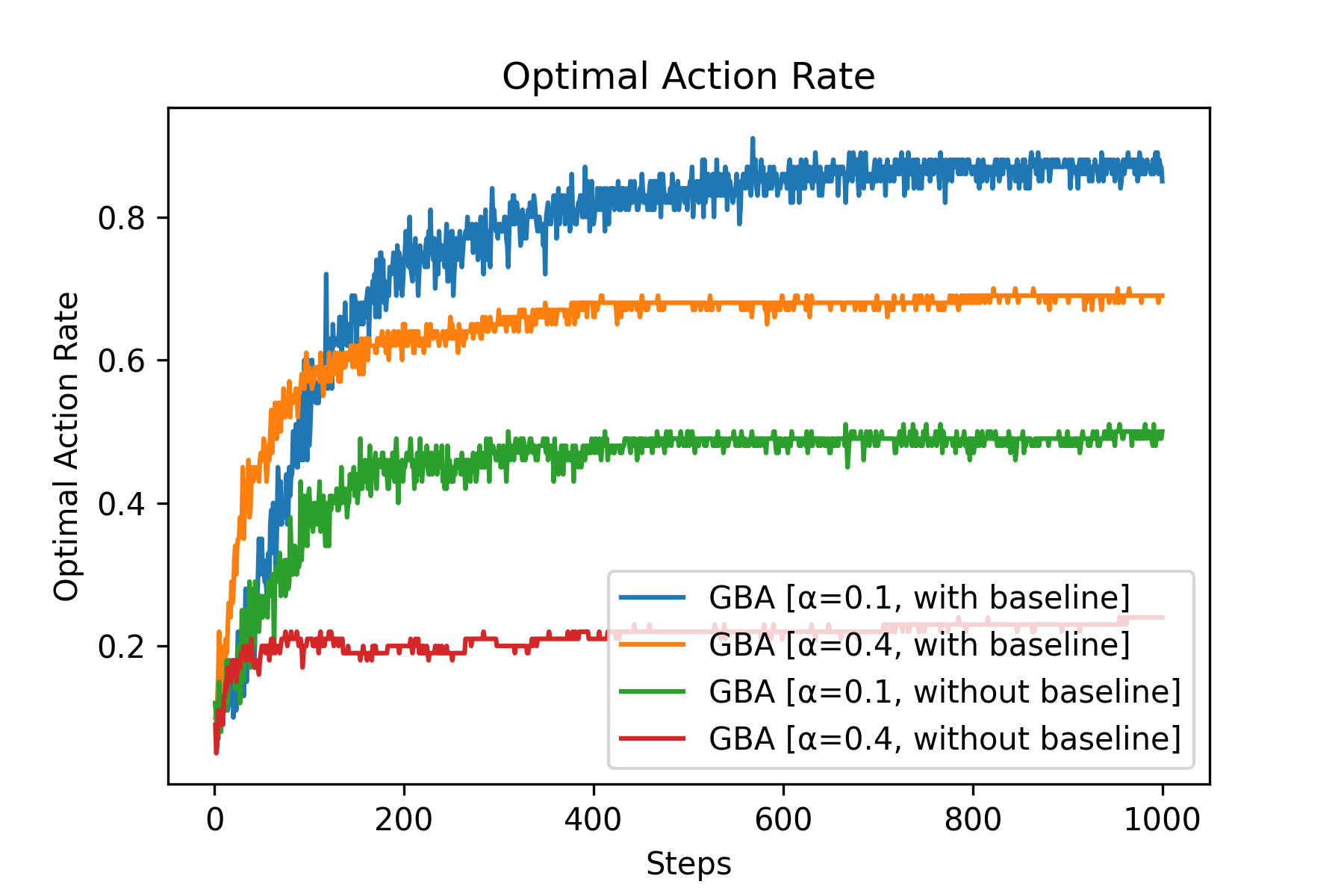
Fig.06 Optimal Action Rate (예시)
$α = 0.1$ 인 경우와 $α = 0.4$ 인 경우, `use_baseline = True`인 경우와 `use_baseline = False`를 조합한 4가지 Gradient Bandit Algorithm을 사용하는 에이전트들의 최적 행동 선택 비율 (k=10, steps=1000, repeats=100)

정상적인 Gradient Bandit Algorithm의 경우 ${\bar{R}}_{t}$ 의 존재 덕분에 $q_{*} (a)$ 가 평균 4인 정규분포에서 추출됐어도 정상적으로 잘 작동한다. 하지만 위 그래프에서 볼 수 있듯이 베이스라인( ${\bar{R}}_{t}$ )을 사용하지 않게 한 에이전트는 성능이 낮게 나온다.

심화 : Gradient Bandit Algorithm의 선호도 업데이트 식 유도 과정

각 행동의 시행 확률 $π_{t} (x)$ 가 주어졌을 때, Gradient Bandit Algorithm의 "성능"은 보상의 기댓값으로 정의할 수 있다(= 성능이 좋을수록 기대할 수 있는 보상의 크기가 크다).

E [R_{t}] = \sum_{x} π_{t} (x) q_{*} (x)

Gradient Ascent를 이용하면 성능을 최대화하는 선호도를 찾을 수 있다.

H_{t + 1} (a) = H_{t} (a) + α \frac{\partial E [R_{t}]}{\partial H_{t} (a)}

이를 전개해보자.

\begin{aligned} H_{t + 1} (a) & = H_{t} (a) + α \frac{\partial E [R_{t}]}{\partial H_{t} (a)} \\ = H_{t} (a) + α \frac{\partial}{\partial H_{t} (a)} [\sum_{x} π_{t} (x) q_{*} (x)] \\ = H_{t} (a) + α \sum_{x} q_{*} (x) \frac{\partial π_{t} (x)}{\partial H_{t} (a)} \end{aligned}

이때

\sum_{x} \frac{\partial π_{t} (x)}{\partial H_{t} (a)} = \frac{\partial}{\partial H_{t} (a)} [\sum_{x} π_{t} (x)] = \frac{\partial}{\partial H_{t} (a)} [1] = 0

이므로, 위 식에 다음과 같이 베이스라인(baseline) 항 $B_{t}$ 를 추가할 수 있다(단, 베이스라인은 $x$ 와 관련없는 스칼라 값이다).

\begin{aligned} H_{t + 1} (a) & = H_{t} (a) + α \sum_{x} q_{*} (x) \frac{\partial π_{t} (x)}{\partial H_{t} (a)} \\ = H_{t} (a) + α \sum_{x} (q_{*} (x) - B_{t}) \frac{\partial π_{t} (x)}{\partial H_{t} (a)} \\ = H_{t} (a) + α \sum_{x} (q_{*} (x) - B_{t}) \frac{\partial π_{t} (x)}{\partial H_{t} (a)} \frac{π_{t} (x)}{π_{t} (x)} \\ = H_{t} (a) + α \sum_{x} π_{t} (x) (q_{*} (x) - B_{t}) \frac{\partial π_{t} (x)}{\partial H_{t} (a)} \frac{1}{π_{t} (x)} \end{aligned}

이때 위 식의 빨간색 테두리 영역은 가능한 모든 행동 $A_{t}$ 에 대해, $A_{t}$ 가 일어날 확률 $π_{t} (A_{t})$ 와 $(q_{*} (A_{t}) - B_{t}) \frac{\partial π_{t} (A_{t})}{\partial H_{t} (a)} \frac{1}{π_{t} (A_{t})}$ 를 곱한, 일종의 기댓값이라 이해할 수 있다. 즉,

\sum_{x} π_{t} (x) (q_{*} (x) - B_{t}) \frac{\partial π_{t} (x)}{\partial H_{t} (a)} \frac{1}{π_{t} (x)} = E [(q_{*} (A_{t}) - B_{t}) \frac{\partial π_{t} (A_{t})}{\partial H_{t} (a)} \frac{1}{π_{t} (A_{t})}]

이라 쓸 수 있다. 또한 $1_{a = x}$ 를 $a = x$ 일 때 1, $a \neq x$ 일 때 0이 되는 확률변수라 하면

\begin{aligned} \frac{\partial π_{t} (A_{t})}{\partial H_{t} (a)} & = \frac{\partial}{\partial H_{t} (a)} [\frac{e^{H_{t} (A_{t})}}{\sum_{b = 1}^{k} e^{H_{t} (b)}}] \\ = \frac{e^{H_{t} (A_{t})} \cdot \frac{\partial H_{t} (A_{t})}{\partial H_{t} (a)} \cdot \sum_{b = 1}^{k} e^{H_{t} (b)} - e^{H_{t} (A_{t})} \cdot \frac{\partial}{\partial H_{t} (a)} [\sum_{b = 1}^{k} e^{H_{t} (b)}]}{{(\sum_{b = 1}^{k} e^{H_{t} (b)})}^{2}} \\ = \frac{e^{H_{t} (A_{t})} \cdot 1_{a = A_{t}}}{\sum_{b = 1}^{k} e^{H_{t} (b)}} - \frac{e^{H_{t} (A_{t})} \cdot e^{H_{t} (a)}}{{(\sum_{b = 1}^{k} e^{H_{t} (b)})}^{2}} \\ = π_{t} (A_{t}) 1_{a = A_{t}} - π_{t} (A_{t}) π_{t} (a) \\ = π_{t} (A_{t}) (1_{a = A_{t}} - π_{t} (a)) \end{aligned}

이므로,

\begin{aligned} H_{t + 1} (a) & = H_{t} (a) + α \sum_{x} π_{t} (x) (q_{*} (x) - B_{t}) \frac{\partial π_{t} (x)}{\partial H_{t} (a)} \frac{1}{π_{t} (x)} \\ = H_{t} (a) + α E [(q_{*} (A_{t}) - B_{t}) \cdot π_{t} (A_{t}) (1_{a = A_{t}} - π_{t} (a)) \cdot \frac{1}{π_{t} (A_{t})}] \\ = H_{t} (a) + α E [(q_{*} (A_{t}) - B_{t}) (1_{a = A_{t}} - π_{t} (a))] \end{aligned}

가 된다. 이때 우리는 $q_{*} (A_{t})$ 를 바로 알 순 없지만, 실험을 통해 받는 보상의 기댓값으로 이를 추정할 수 있다. 이를 수식으로 나타내면 다음과 같다.

q_{*} (A_{t}) = E [R_{t} | A_{t}]

또한 베이스라인으로 $A_{t}$ 에 의존하지 않는 값인 ${\bar{R}}_{t}$ 를 사용할 수 있다.

\begin{aligned} H_{t + 1} (a) & = H_{t} (a) + α E [(q_{*} (A_{t}) - B_{t}) (1_{a = A_{t}} - π_{t} (a))] \\ = H_{t} (a) + α E [(E [R_{t} | A_{t}] - {\bar{R}}_{t}) (1_{a = A_{t}} - π_{t} (a))] \end{aligned}

그런데 Gradient Ascent Algorithm에서는 한 번 시행 후 이 결과값을 바탕으로 바로 선호도 업데이트를 진행한다(= Stochastic Gradient Ascent를 수행한다). 즉 기댓값을 계산할 때 사용하는 데이터의 양이 1개이므로 기댓값 함수를 바로 풀어버릴 수 있다. 이를 이용해 위 식을 정리하면 다음과 같이 된다.

\begin{aligned} H_{t + 1} (a) & = H_{t} (a) + α E [(E [R_{t} | A_{t}] - {\bar{R}}_{t}) (1_{a = A_{t}} - π_{t} (a))] \\ = H_{t} (a) + α (R_{t} - {\bar{R}}_{t}) (1_{a = A_{t}} - π_{t} (a)) \end{aligned}

∴ {\begin{cases} H_{t + 1} (a) = H_{t} (a) + α (R_{t} - {\bar{R}}_{t}) (1 - π_{t} (a)) & (if a = A_{t}) \\ H_{t + 1} (a) = H_{t} (a) - α (R_{t} - {\bar{R}}_{t}) π_{t} (a) & (if a \neq A_{t}) \end{cases}

이렇게 Gradient Ascent Algorithm의 선호도 업데이트 식을 유도할 수 있다.

눈치챘겠지만 사실 베이스라인 $B_{t}$ 은 모든 행동 $x$ 에 대해서 독립적이기만 하면 된다. 즉 $B_{t}$ 로 그냥 0을 사용해도 되고, 아무런 숫자(1000)를 써도 된다는 것이다. 하지만 적절한 값을 베이스라인으로 사용하면 선호도 $H_{t} (a)$ 의 수렴 속도를 빠르게 할 수 있다. 평균 보상( ${\bar{R}}_{t}$ )은 최고의 선택이 아닐 순 있지만, 계산하기 쉽고 꽤 잘 작동하는 베이스라인이다.

확장 : Associative Search (Contextual Bandits)

우리가 이때까지 풀었던 k-armed Bandit Problem을 Nonassociative Task라 한다. Nonassociative Task란 현재 상황(state)과 행동을 연결(association)할 필요가 없는 문제를 뜻한다. k-armed Bandit Problem에서는 특정 행동을 해도 문제 상황(= 상태)이 안 바뀌기 때문에^[14], k-armed Bandit Problem에서는 이전에 받은 보상을 바탕으로 다음 행동을 결정하기만 하면 됐다.

그렇다면 여러 개의 k-armed Bandit Problem을 동시에 푸는 상황을 생각해 보자. 이를테면 슬롯 머신이 10개씩 놓여 있는 6개의 방이 있을 때, 주사위를 굴려 나온 숫자에 해당하는 방에 들어가 원하는 슬롯머신을 당기는 과정을 100번 수행해 최대한 많은 상금을 받으려 하는 문제를 생각해 보자. 이 문제에서는 "주사위를 굴려 나온 수"라는, 현재 상황(situation)을 추가로 고려해야 한다. 즉 이 문제를 풀 때는 "어떠어떠한 상황에서, 어떠어떠한 행동을 하겠다"는, 정책(policy)을 만들어야 한다. 이 문제같은 경우 정책을 만들기 비교적 쉽다. "주사위를 굴려 나온 수"라는, 현재 상태를 구별할 수 있는 명확한 단서가 있기에 이 값을 기준으로 정책을 만들면 된다.^[15] 이런 식의 문제를 Associative Task라 한다. 그리고 Associative Task를 푸는 과정을 Associative Search 또는 Contextual Bandits이라 한다.

실제 RL 문제는 여기에서 한 걸음 더 나간다. 위 문제에서 특정 방에 들어가 특정 슬롯머신을 당기는 행동은 보상은 만들어 내지만 현재 상태(state)에 아무런 영향을 끼치지 않는다. 하지만 실제 RL 문제에서 특정 행동을 하는 것은 보상을 만들 뿐만 아니라 자신을 둘러싸고 있는 환경의 상태에도 영향을 미친다.

결론

우리는 k-armed Bandit Problem을 해결하는 다양한 방법들을 살펴보았다. 결국 관건은 어떤 비율로 Exploration과 Exploitation을 할 것인가이다.

$ε$ -greedy Method : 간혹( $ε$ 의 확률로) 완전 무작위로 다음 행동을 선택한다.
Optimistic Initial Values : 행동의 가치 추정값의 초기값으로 낙관적인(optimistic) 값을 사용해 탐색 비율을 늘릴 수 있다.
UCB Action Selection : UCB가 높은 행동을 결정론적으로(deterministically) 선택한다. 아직 여러번 시행되지 않은 행동은 UCB가 높다.
Gradient Bandit Algorithm : 각 행동의 선호도(preference)를 기반으로 다음 행동을 확률적으로 선택한다.

그렇다면 위 네 가지 방법 중 어떤 방법이 k-armed Bandit Problem을 해결하는 가장 좋은 방법일까? 사실 각 방법들은 독자적인 파라미터를 사용하기에 이들을 바로 비교하는 것은 어렵다. 이들을 비교하는 한 가지 방법으로 각 방법별로 학습 곡선(learning curve)을 그린 후 이를 비교하는 방법이 있다. 학습 곡선이란 여러 개의 파라미터 값들에 대해 목표값을 그래프로 나타낸 것을 말한다. 모든 파라미터에 대해 학습 곡선을 그리면 또 비교가 어려워지므로, 위 네 가지 방법 각각 핵심 파라미터( $ε$ , $Q_{1} (a)$ , $c$ , $α$ )를 바꿔가며 평균 보상^[16]을 계산하자. 이를 그래프로 나타내면 Fig.07과 같이 된다(참고로 이렇게 그린 그래프를 Parameter Study라 한다).

Code : Parameter Study

python

import numpy as np
from matplotlib import pyplot as plt
from abc import *

class Agent(metaclass=ABCMeta):
    def __init__(self, k):
        self.k = k
        self.reward = 0
    
    @abstractmethod
    def chooseAction(self, t):
        pass
    
    def train(self, reward):
        self.reward += reward
    
    def getReward(self):
        return self.reward
    
    @abstractmethod
    def getName(self):
        pass
    
class EpsilonGreedyMethod(Agent):
    def __init__(self, k, epsilon):
        super().__init__(k)
        self.epsilon = epsilon
        self.count = np.zeros(self.k, dtype=int)
        self.estimated_values = np.zeros(self.k, dtype=float)
        
    def chooseAction(self, t):
        if np.random.random() < self.epsilon: # exploration
            return np.random.choice(self.k)
        else: # exploitation
            max_actions = np.argwhere(self.estimated_values == np.max(self.estimated_values)).flatten()
            return np.random.choice(max_actions)
    
    def train(self, action, reward):
        super().train(reward)
        self.count[action] += 1
        self.estimated_values[action] = self.estimated_values[action] + (1/self.count[action]) * (reward - self.estimated_values[action])    
        
    def getName(self):
        return f"ε-greedy Method [ε={self.epsilon}]"
    
class GreedyMethod(Agent):
    def __init__(self, k, q1=0):
        super().__init__(k)
        self.q1 = q1
        self.count = np.zeros(self.k, dtype=int)
        self.estimated_values = np.full(shape=self.k, fill_value=self.q1, dtype=float)
        
    def chooseAction(self, t):
        max_actions = np.argwhere(self.estimated_values == np.max(self.estimated_values)).flatten()
        return np.random.choice(max_actions)
    
    def train(self, action, reward):
        super().train(reward)
        self.count[action] += 1
        self.estimated_values[action] = self.estimated_values[action] + 0.1 * (reward - self.estimated_values[action])    
        
    def getName(self):
        return f"Greedy Method with Optimistic Initial Values [α=0.1, q1={self.q1}]"
        
class UCB(Agent):
    def __init__(self, k, c):
        super().__init__(k)
        self.c = c
        self.count = np.zeros(self.k, dtype=int)
        self.estimated_values = np.zeros(self.k, dtype=float)
        
    def chooseAction(self, t):
        never_tried_actions = np.where(self.count == 0)[0]
        
        if len(never_tried_actions) != 0:
            return np.random.choice(never_tried_actions)
        
        ucb = self.estimated_values + self.c * np.sqrt((np.log(t))/(self.count))
        max_actions = np.argwhere(ucb == np.max(ucb)).flatten()
        return np.random.choice(max_actions)
    
    def train(self, action, reward):
        super().train(reward)
        self.count[action] += 1
        self.estimated_values[action] = self.estimated_values[action] + (1/self.count[action]) * (reward - self.estimated_values[action])    
    
    def getName(self):
        return f"UCB [c={self.c}]"

    
class GradientBanditAlgorithm(Agent):
    def __init__(self, k, alpha):
        super().__init__(k)
        self.alpha = alpha
        self.H = np.zeros(self.k, dtype=float)
        self.baseline = 0
        self.count = 0
    
    def _getPi(self):
        powers = np.exp(self.H)
        return powers/np.sum(powers)
    
    def chooseAction(self, t):
        return np.random.choice(self.k, p=self._getPi())
    
    def train(self, action, reward):
        super().train(reward)
        indicator = np.zeros(self.k, dtype=int)
        indicator[action] = 1
        self.H = self.H + self.alpha * (reward - self.baseline) * (indicator - self._getPi())
        
        self.count += 1
        self.baseline = self.baseline + (1/self.count) * (reward - self.baseline)
    
    def getName(self):
        return f"GBA [α={self.alpha}]"

class Testbed:
    def __init__(self, k, mean=0, std=1):
        self.true_values = np.random.normal(size=k, loc=mean, scale=std)
        self.k = k
    
    def sample(self, action, std=1):
        assert action in range(self.k), "Invalid param:action"
        return np.random.normal(loc=self.true_values[action], scale=std)
    
    def getTrueValues(self):
        return self.true_values

steps = 1000
repeats = 100
k = 10
values = [1/128, 1/64, 1/32, 1/16, 1/8, 1/4, 1/2, 1, 2, 4]

rewards_total = {}

# Epsilon-Greedy Method
avg_rewards = np.zeros(len(values), dtype=float)
for repeat in range(repeats):
    testbed = Testbed(k=k)
    for i, epsilon in enumerate(values):
        agent = EpsilonGreedyMethod(k=k, epsilon=epsilon)
        for step in range(steps):
            action = agent.chooseAction(step)
            sample = testbed.sample(action=action)
            agent.train(action=action, reward=sample)
            
        avg_rewards[i] += agent.getReward() / steps

avg_rewards = avg_rewards / repeats
rewards_total["EpsilonGreedyMethod"] = avg_rewards

# Greedy Method with Optimistic Initial Values
avg_rewards = np.zeros(len(values), dtype=float)
for repeat in range(repeats):
    testbed = Testbed(k=k)
    for i, q1 in enumerate(values):
        agent = GreedyMethod(k=k, q1=q1)
        for step in range(steps):
            action = agent.chooseAction(step)
            sample = testbed.sample(action=action)
            agent.train(action=action, reward=sample)
            
        avg_rewards[i] += agent.getReward() / steps

avg_rewards = avg_rewards / repeats
rewards_total["GreedyMethod"] = avg_rewards

# UCB Action Selection
avg_rewards = np.zeros(len(values), dtype=float)
for repeat in range(repeats):
    testbed = Testbed(k=k)
    for i, c in enumerate(values):
        agent = UCB(k=k, c=c)
        for step in range(steps):
            action = agent.chooseAction(step)
            sample = testbed.sample(action=action)
            agent.train(action=action, reward=sample)
            
        avg_rewards[i] += agent.getReward() / steps

avg_rewards = avg_rewards / repeats
rewards_total["UCB"] = avg_rewards

# Gradient Bandit Algorithm
avg_rewards = np.zeros(len(values), dtype=float)
for repeat in range(repeats):
    testbed = Testbed(k=k)
    for i, alpha in enumerate(values):
        agent = GradientBanditAlgorithm(k=k, alpha=alpha)
        for step in range(steps):
            action = agent.chooseAction(step)
            sample = testbed.sample(action=action)
            agent.train(action=action, reward=sample)
            
        avg_rewards[i] += agent.getReward() / steps

avg_rewards = avg_rewards / repeats
rewards_total["GradientBanditAlgorithm"] = avg_rewards

# Draw Graph
plt.plot(values[0:6], rewards_total["EpsilonGreedyMethod"][0:6], label="Epsilon Greedy Method")
plt.plot(values[5:10], rewards_total["GreedyMethod"][5:10], label="Greedy Method with Optimistic Initial Values")
plt.plot(values[3:10], rewards_total["UCB"][3:10], label="UCB Action Selection")
plt.plot(values[2:9], rewards_total["GradientBanditAlgorithm"][2:9], label="Gradient Bandit Algorithm")
plt.xlabel("values")
plt.ylabel("Average Reward")
plt.title("k-armed Bandit Problem - Parameter Study")
plt.xscale("log")
plt.xticks(values, ["1/128", "1/64", "1/32", "1/16", "1/8", "1/4", "1/2", "1", "2", "4"])
plt.minorticks_off()
plt.legend(bbox_to_anchor=(1, 1))
plt.show()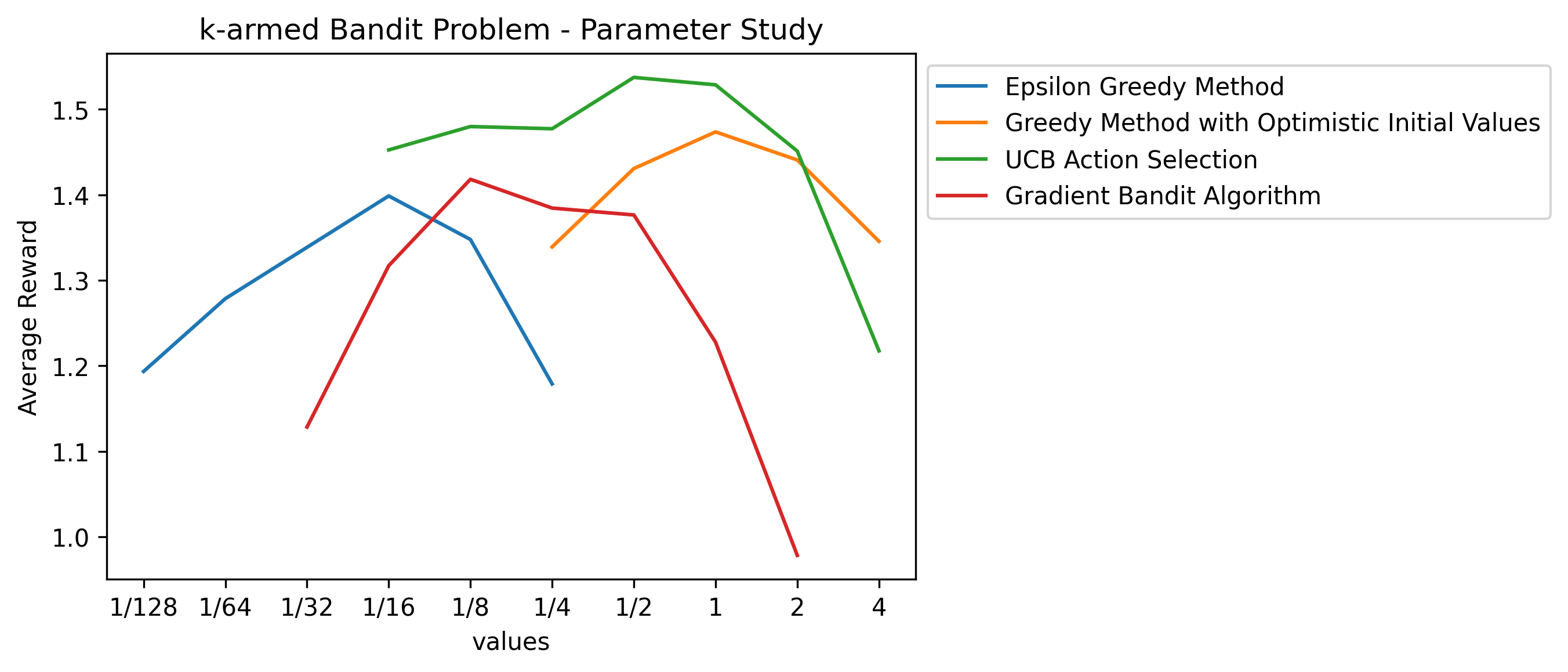

1
2
3
4
5
6
7
8
9
10
11
12
13
14
15
16
17
18
19
20
21
22
23
24
25
26
27
28
29
30
31
32
33
34
35
36
37
38
39
40
41
42
43
44
45
46
47
48
49
50
51
52
53
54
55
56
57
58
59
60
61
62
63
64
65
66
67
68
69
70
71
72
73
74
75
76
77
78
79
80
81
82
83
84
85
86
87
88
89
90
91
92
93
94
95
96
97
98
99
100
101
102
103
104
105
106
107
108
109
110
111
112
113
114
115
116
117
118
119
120
121
122
123
124
125
126
127
128
129
130
131
132
133
134
135
136
137
138
139
140
141
142
143
144
145
146
147
148
149
150
151
152
153
154
155
156
157
158
159
160
161
162
163
164
165
166
167
168
169
170
171
172
173
174
175
176
177
178
179
180
181
182
183
184
185
186
187
188
189
190
191
192
193
194
195
196
197
198
199
200
201
202
203
204
205
206
207
208
209
210
211
212
213

Fig.07 Parameter Study (예시)
위에서 학습한 k-armed Bandit Problem을 푸는 네 가지 방법들에 대한 Parameter Study

위 그래프를 보면 모든 방법들의 그래프가 ∩ 모양을 띄고 있음을 볼 수 있다. 이는 모든 방법들이 극단적으로 크거나 극단적으로 작은 파라미터에서는 좋은 성능을 보이지 못한다는 것을 보여준다. 위 그래프에 의하면 UCB Action Selection이 가장 좋은 성능을 보인다고 할 수 있겠다.

많은 책이나 블로그에서 k-armed Bandit Problem을 잘못 해석해 "외팔이 강도(One-armed Bandit)가 k개의 슬롯머신을 당길 때 보상을 최대화하는 문제"라 설명을 하는데, 사실 one-armed bandit는 미국에서는 슬롯 머신을 부르는 속어이다(팔 하나(레버)를 달고 당신을 털어가기 때문). k-armed Bandit Problem은 여기에서 이름을 따온 것이다. 즉 k-armed Bandit Problem이라 하면 (정상적인 사람이) 레버가 k개 있는 슬롯 머신에서, k개의 레버 중 하나를 골라 당기는 과정을 여러 번 반복할 때 받을 전체 보상을 최대화하는 문제를 뜻한다. ↩︎
탐욕적 행동이 아닌 행동 ↩︎
이 과정에서 탐욕적 행동이 바뀔 수도 있다. ↩︎
$Q_{n - 1}$ 이 아닌 $Q_{n}$ 인 이유는 다음과 같다: Sample-average Method는 이전 결과들로부터 각 행동의 가치를 추정하고, 이를 기반으로 행동을 결정하고, 결정한 행동을 수행해 보상을 받는 과정을 반복하는 것이다. 이때 시점 $n - 1$ 에서 받은 $n - 1$ 번째 보상을 이용해 가치를 업데이트하는 것은 시점 $n$ 일 때이므로 $Q_{n - 1}$ 이 아닌 $Q_{n}$ 라 하는 것이다. ↩︎
그래서 이를 강조하여 k-armed Bandit Problem을 Stationary Bandit Problem이라 부르기도 한다. ↩︎
$0^{0} = 1$ 로 계산한다. ↩︎
수렴하지 않기에 확률 분포가 고정되어 있지 않는 상황(nonstationary)에서도 잘 작동하는 것이다. ↩︎
$\sum_{n = 1}^{\infty} \frac{1}{n} = \infty$ , $\sum_{n = 1}^{\infty} {(\frac{1}{n})}^{2} = \frac{π^{2}}{6}$ ↩︎
사실 우리가 "+5"를 낙관적인 값으로 선택할 수 있었던 것은 이미 $q_{*} (a)$ 가 평균 0, 분산 1인 정규분포를 따른다는 사전 지식을 알고 있었기 때문에 가능했다. 즉 크게 보면 Optimistic Initial Values도 사전 지식을 $Q_{1}$ 에 담은 것이라 할 수 있다. ↩︎
사실 Nonstationary Problem을 풀 때는 초기값을 어떻게 설정하던지 크게 도움이 안 된다. ↩︎
$Q_{t} (a)$ 의 값이 큰 행동 $a$ 를 선택 ↩︎
단, ${\bar{R}}_{1} = R_{1}$ ↩︎
Softmax function에서 $e^{H_{t} (a) + 1000} = e^{1000} \cdot e^{H_{t} (a)}$ 이므로 $e^{1000}$ 이 모두 약분된다. ↩︎
첫 번째로 슬롯을 당길 때와 100번째로 슬롯을 당길 때의 상황이 같다. ↩︎
ex) "1번 방에서는 4번 슬롯머신을 당긴다. 2번 방에서는 9번 슬롯머신을 당긴다. ..., 6번 방에서는 1번 슬롯머신을 당긴다." ↩︎
평균 보상은 다음과 같이 계산한다: 한 Testbed에 대해 1,000스탭 시뮬레이션을 돌려, 각 스탭마다 받는 보상의 평균값을 구하는 과정을 100번 시행. 그렇게 나온 평균 보상들의 평균. ↩︎

L03. Multi-armed Bandits

k-armed Bandit Problem ​

Action-value Method ​

Sample-average Method ​

ε-greedy Method ​

Incremental Implementation ​

여담 : Qn+1=Qn+α(Rn−Qn) ​

구현 ​

Nonstationary Bandit Problem ​

Exponential Recency-weighted Average Method ​

여담 : Qn+1=Qn+α(Rn−Qn)가 수렴할 α의 조건 ​

Optimistic Initial Values ​

UCB(Upper-Confidence-Bound) Action Selection ​

Gradient Bandit Algorithm ​

확장 : Associative Search (Contextual Bandits) ​

결론 ​

k-armed Bandit Problem

Action-value Method

Sample-average Method

ε-greedy Method

Incremental Implementation

여담 : $Q_{n + 1} = Q_{n} + α (R_{n} - Q_{n})$

구현

Nonstationary Bandit Problem

Exponential Recency-weighted Average Method

여담 : $Q_{n + 1} = Q_{n} + α (R_{n} - Q_{n})$ 가 수렴할 $α$ 의 조건

Optimistic Initial Values

UCB(Upper-Confidence-Bound) Action Selection

Gradient Bandit Algorithm

확장 : Associative Search (Contextual Bandits)

결론