MC Method(Monte Carlo Method)란?

이전 글에서 우리는 DP에 대해 배웠다. DP의 핵심 아이디어 중 하나는 GPI이다. GPI란 현재 정책으로부터 가치 함수를 계산하는 Evaluation 과정과 현재 가치 함수로부터 개선된 정책을 계산하는 Improvement 과정을 번갈아가며 진행해 최적 정책과 최적 가치 함수를 찾는 방법을 말한다. DP에서는 환경에 대한 지식을 완벽히 알고 있는 상황을 가정하기에 Evaluation 과정과 Improvement 과정을 계산(compute) 할 수 있었다.

그러나 당연히 대부분의 RL 문제에서는 환경에 대한 지식을 완벽하게 알 수 없으므로, 최적 정책을 찾기 위해 DP를 사용할 수 없다. 하지만 이런 상황에서도 최적 정책을 찾을 수 있는 방법이 있으니, 바로 MC Method(Monte Carlo Method)이다.

일반적으로 MC Method는 추정값을 무작위적인 방법으로 추정하는 알고리즘을 의미한다. RL에서의 MC Method도 비슷한 의미를 가지고 있다. RL에서의 MC Method는 경험(experience)^[1]^[2]으로부터 최적 정책, 최적 가치 함수 등을 추정하는 방법을 의미한다. 조금 더 구체적으로 말하면, MC Method는 GPI의 아이디어를 사용해 Sample Return^[3]들의 평균으로부터 최적 가치 함수, 최적 정책 등을 찾는 방법을 의미한다.

한 에피소드가 끝나야 Sample Return을 계산 가능하기 때문에, MC Method는 Episodic Task에 대해서만 사용되고,^[4] 가치 함수와 정책 등은 반드시 한 에피소드가 종료되어야 업데이트된다.^[5]

여담 : k-armed Bandit Problem와의 관련성

사실 우리는 k-armed Bandit Problem에서 MC Method와 비슷한 방법을 이미 보았다. 관측 결과를 평균낸 값을 추정치로 사용하는 MC Method는 Sample-average Method와 매우 유사하다. 차이점은, Sample-average Method에서는 보상(reward) 들의 평균을 계산해 추정값으로 사용하지만, MC Method에서는 Return들의 평균을 계산해 추정값으로 사용한다. 또한 MC Method는 MDP 등 범용적인 문제에 적용할 수 있지만, Sample-average Method는 k-armed Bandit Problem에만 쓸 수 있다. Sample-average Method에서는 상태(state)에 대한 고려가 없기 때문이다.

굳이 끼워맞추자면 MC Method는 각 상태가 각기 다른 k-armed Bandit Problem인 문제를 푸는 Associative Search이라 할 수 있다. 이때 한 상태에서 어떤 행동을 했을 때의 Return은 이후 상태에서 어떤 행동을 했는지에 따라 영향을 받으므로, 각 k-armed Bandit Problem은 Nonstationary Problem이 된다.

MC Prediction(Monte Carlo Prediction)

우선 MC Method를 이용해 Prediction 문제(주어진 정책에 대한 가치 함수 계산)를 풀어보자. MC Method를 이용해 주어진 정책 $π$ 의 가치 함수를 추정(학습)하는 것을 MC Prediction(Monte Carlo Prediction) 이라 한다. 이는 GPI에서 Evaluation 과정에 해당된다. MC Prediction의 방법은 엄청 간단하다. 가치 함수는 Return의 기댓값이므로, 여러 번의 시뮬레이션을 수행해 관측된 Return들의 평균을 구하면 된다. 더 많은 Return이 관측될수록 추정한 가치 함수는 점점 더 정확해 진다.

가치 함수에는 상태-가치 함수(state-value function) $v_{π}$ 와 행동-가치 함수(action-value function) $q_{π}$ , 이렇게 두 종류가 있다. 각각을 추정하는 방법을 좀 더 자세히 알아보자.

$v_{π}$ 추정하기

우선 방문했다(visit) 라는 용어를 정의하자. 어떤 에피소드에 특정 상태 $s$ 가 등장한 것을 $s$ 에 방문했다(visit) 하고, $s$ 에 처음 방문했을 때를 $s$ 에 최초방문했다(first-visit) 고 한다.

그렇다면 다음 두 가지 방법을 생각할 수 있다.

First-visit MC Prediction : 상태 $s$ 에 최초방문(first-visit)했을 때 받는 Return들의 평균으로 $v_{π} (s)$ 를 추정하는 방법
Every-visit MC Prediction : 상태 $s$ 에 방문(visit)했을 때 받는 Return들의 평균으로 $v_{π} (s)$ 를 추정하는 방법

두 방법 모두 최초방문 및 방문 횟수가 커지면 커질수록 참값( $v_{π} (s)$ )에 수렴하게 된다.^[6]

First-visit MC Prediction을 의사 코드(pseudo code)로 나타내면 다음과 같다.

Pseudo Code : First-visit MC Prediction

입력 : 정책 $π$

1. 초기화

모든 $s \in S$ 에 대해, $V (s) \in R$ 을 임의의 값으로 초기화

모든 $s \in S$ 에 대해, Returns( $s$ ) = [] (빈 리스트)로 초기화

2. 추정

Loop forever (for each episode):

$π$ 를 따라 에피소드 생성 : $S_{0}, A_{0}, R_{1}, S_{1}, A_{1}, R_{2}, \dots, S_{T - 1}, A_{T - 1}, R_{T}$

$G \leftarrow 0$

Loop for each step of episode, $t = T - 1, T - 2, \dots, 0$ :

$G \leftarrow γ G + R_{t + 1}$

If not $S_{t}$ appears in $S_{0}, S_{1}, \dots, S_{t - 1}$ :

Returns( $S_{t}$ ).append( $G$ )

$V (S_{t}) \leftarrow$ average(Returns( $S_{t}$ ))

예시 : BlackJack

블랙잭 게임에서 First-visit MC Prediction을 이용해 $v_{π}$ 를 추정해 보자. 블랙잭 게임의 규칙은 다음과 같다.

Blackjack

블랙잭은 플레이어와 딜러가 각각 점수의 총합이 21을 넘지 않는 선에서 점수를 최대한 크게 하는 것을 목표로 싸우는 카드 게임이다. 세부 규칙은 다음과 같다.

숫자 카드의 점수는 카드에 적힌 숫자로 계산한다. 얼굴 카드(J, Q, K)의 점수는 모두 10점으로 계산한다. 에이스 카드(A)는 1점 혹은 11점으로 계산할 수 있다.
게임이 시작되면 딜러는 플레이어와 본인 앞에 각각 두 장씩의 카드를 준다. 이때 딜러의 카드 중 한 장은 숨겨져 있다(facing down). 나머지 카드 3장은 모두 공개되어 있다(facing up).
플레이어가 카드를 배분받는 즉시 21점을 달성한 경우(즉, 에이스 카드 한 장과 10점짜리 카드 한 장을 받았다면) 이를 natural이라 한다. 이 경우 플레이어는 딜러가 natural이지 않는 이상 즉시 승리한다. 만약 딜러도 natural이면 비긴 것이다.
natural이 아닌 경우, 플레이어는 추가적인 카드를 한 장씩 계속 요청할 수 있다(이를 hit이라 한다). 플레이어는 더 이상 카드를 받길 원하지 않거나(이를 stick이라 한다) 21점을 초과할 때까지(이를 bust라 한다) hit할 수 있다.
bust가 되면 플레이어는 즉시 진다.
플레이어가 적절한 시점에서 stick을 하면 딜러가 카드를 받을 차례가 된다. 딜러는 정해진 규칙(현재 점수가 17점보다 낮으면 hit하고, 17점보다 크거나 같으면 stick한다)에 따라 카드를 받는다. 이때 만약 딜러가 bust가 되면 플레이어는 즉시 이긴다. bust가 나지 않으면 21점에 더 가까운 쪽이 승리한다. 만약 둘의 점수가 같다면 비긴 것이다.

이제 다음을 가정해 블랙잭을 Episodic Finite MDP로 만들자.

각 판은 하나의 독립적인 에피소드이다. 각 에피소드마다 새로운 덱(deck)을 쓴다.^[7]
승리 시 +1, 패배 시 -1, 비길 시 0의 보상을 받는다. 게임 진행 중에는 아무런 보상을 받지 않는다.
$γ = 1$ ^[8]
$A$ = { hit, stick }
$S$ = { (agent_sum, dealer_showing, is_usable) | 12 ≤ agent_sum ≤ 21, 2 ≤ dealer_showing ≤ 11, is_usable ∈ { True, False } }^[9]
- agent_sum : 현재 에이전트(플레이어)가 들고 있는 카드들의 점수의 합(12-21)
- dealer_showing : 딜러의 공개된 카드의 점수(ace(11), 2-10)
- is_usable : bust 없이 11점으로 계산될 수 있는 에이스 카드를 들고 있는지 여부(True, False)

이제 정책 $π$ 가 다음과 같이 주어졌다고 해 보자.

$π$ : agent_sum이 20 또는 21인 경우 행동 stick을 선택한다. 나머지 경우 행동 hit을 선택한다.

First-visit MC Prediction을 이용해 $v_{π}$ 를 추정하려면, 우선 정책 $π$ 를 따르면서 여러 번의 시뮬레이션을 진행한다. 그리고 각 상태에 최초방문했을 때의 Return들을 평균한다.

Code : First-visit MC Prediction

python

import numpy as np
import matplotlib.pyplot as plt

class Env:
    def __init__(self):
        self.deck = None
        self.agent_cards = None
        self.dealer_cards = None
        
    def _pop(self):
        card = self.deck[-1]
        self.deck = self.deck[0:-1]
        return card
    
    def _getCardScore(self, card_idx):
        num = card_idx % 13
        if num == 0: # Ace
            return 11
        elif num in [10, 11, 12]: # J, Q, K
            return 10
        else:
            return num + 1
       
    def _getScore(self, cards):
        ace_count = 0
        total_score = 0
        for card in cards:
            score = self._getCardScore(card)
            total_score += score
            if score == 11:
                ace_count += 1
                
        while total_score > 21 and ace_count > 0:
            total_score -= 10
            ace_count -= 1
        
        if ace_count > 0:
            is_usable = True
        else:
            is_usable = False
        
        return total_score, is_usable
    
    def _dealer_playing(self):
        while self._getScore(self.dealer_cards)[0] < 17:
            self.dealer_cards.append(self._pop())
        
    def _getState(self):
        agent_sum, is_usable = self._getScore(self.agent_cards)
        dealer_showing = self._getCardScore(self.dealer_cards[0])
        return agent_sum, dealer_showing, is_usable
    
    def newGame(self):
        self.deck = np.arange(52, dtype=int)
        np.random.shuffle(self.deck)
        
        self.agent_cards = [self._pop() for x in range(2)]
        self.dealer_cards = [self._pop() for x in range(2)]
        
        if self._getScore(self.agent_cards)[0] == 21:
            if self._getScore(self.dealer_cards)[0] == 21:
                return 1, self._getState(), 0
            else:
                return 1, self._getState(), 1
        else:
            return 0, self._getState(), 0
                
    def interact(self, action):
        if action == "hit":
            self.agent_cards.append(self._pop())
            if self._getScore(self.agent_cards)[0] > 21: # agent bust
                return 1, self._getState(), -1
            else:
                return 0, self._getState(), 0
        else: # stick
            self._dealer_playing()
            agent_score = self._getScore(self.agent_cards)[0]
            dealer_score = self._getScore(self.dealer_cards)[0]
            
            if dealer_score > 21: # dealer bust
                return 1, self._getState(), 1
            else:
                if agent_score > dealer_score:
                    return 1, self._getState(), 1
                elif agent_score < dealer_score:
                    return 1, self._getState(), -1
                else:
                    return 1, self._getState(), 0

class Agent:
    def action(self, state):
        agent_sum, dealer_showing, is_usable = state
        if agent_sum == 20 or agent_sum == 21:
            return "stick"
        else:
            return "hit"
                
def simulate(trial):
    episodes = []
    
    for t in range(trial):
        agent = Agent()
        env = Env()
        episode = []
        
        status, state, reward = env.newGame()
        episode.append(state)
        
        while status == 0:
            action = agent.action(state)
            episode.append(action)
            
            status, state, reward = env.interact(action)
            episode.append(reward)
            episode.append(state)
        
        episodes.append(episode)
        
    return episodes

def predict(episodes):
    def getStateIdx(state):
        agent_sum, dealer_showing, is_usable = state
        if agent_sum < 12:
            return -1
        else:
            return (1 if is_usable else 0) * 100 + (agent_sum - 12) * 10 + ((dealer_showing - 1) if dealer_showing < 11 else 0)
        
    def parseEpisode(episode):
        R = []
        S = []
        A = []
        
        idx = 0
        
        R.append(None)
        S.append(getStateIdx(episode[idx]))
        idx += 1
        if len(episode) != 1:
            A.append(episode[1])
            idx += 1
        else:
            A.append(None)
            return R, S, A, len(R)
        
        while idx < len(episode) - 2:
            R.append(episode[idx])
            idx += 1
            S.append(getStateIdx(episode[idx]))
            idx += 1
            A.append(episode[idx])
            idx += 1
        
        R.append(episode[idx])
        idx += 1
        S.append(getStateIdx(episode[idx]))
        idx += 1
        A.append(None)
        idx += 1
        
        return R, S, A, len(R)
        
    V = [0 for x in range(200)]
    Returns = [[] for x in range(200)]
    gamma = 1
    
    for episode in episodes:
        R, S, A, T = parseEpisode(episode)
        if T == 1:
            continue
        
        G = 0
        for t in reversed(range(T - 1)):
            G = gamma * G + R[t + 1]
            
            if S[t] == -1:
                continue
            elif not S[t] in S[0:t]:
                Returns[S[t]].append(G)
                V[S[t]] = sum(Returns[S[t]]) / len(Returns[S[t]])
    
    return V

def drawGraph(V):
    agent_sum = np.arange(12, 22)
    dealer_showing = np.arange(1, 11)
    agent_sum_mesh, dealer_showing_mesh = np.meshgrid(agent_sum, dealer_showing)

    no_usable = np.zeros_like(agent_sum_mesh, dtype=float)
    yes_usable = np.zeros_like(agent_sum_mesh, dtype=float)
    for i in range(10):
        for j in range(10):
            no_usable[i, j] = V[10 * j + i]
            yes_usable[i, j] = V[100 + 10 * j + i]

    fig = plt.figure(figsize=(10, 5))
    subplots = [fig.add_subplot(1, 2, 1, projection='3d'), fig.add_subplot(1, 2, 2, projection='3d')]
    subplots[0].plot_surface(dealer_showing_mesh, agent_sum_mesh, no_usable, rstride=1, cstride=1, alpha=0.8, color='red', edgecolor='black')
    subplots[1].plot_surface(dealer_showing_mesh, agent_sum_mesh, yes_usable, rstride=1, cstride=1, alpha=0.8, color='blue', edgecolor='black')
    subplots[0].set_title("No usable")
    subplots[1].set_title("Usable")
    for subplot in subplots:
        subplot.set_xlim(1, 10)
        subplot.set_xticks([1, 10])
        subplot.set_xticklabels(['A', '10'])
        subplot.set_xlabel("Dealer Showing")
        subplot.set_ylim(12, 21)
        subplot.set_yticks([12, 21])
        subplot.set_ylabel("Agent Sum")
        subplot.set_zlim(-1, 1)
        subplot.set_zticks([-1, 1])
        subplot.set_zlabel("Reward")

    plt.show()

if __name__ == "__main__":
    episodes = simulate(10000)
    V = predict(episodes)
    drawGraph(V)
    
    episodes = simulate(500000)
    V = predict(episodes)
    drawGraph(V)

코드 설명

line 4 ~ 88 : 환경(Environment)을 나타내는 클래스
- line 10 ~ 13 : Env._pop()
  - 덱에서 카드 한 장을 꺼내는 메서드
- line 15 ~ 22 : Env._getCardScore()
  - 카드의 인덱스를 받아 점수로 변환하는 메서드
- line 24 ~ 42 : Env._getScore()
  - 들고 있는 패의 점수를 계산하는 메서드
  - 현재 패의 점수, usable ace가 있는지 여부 순으로 반환
- line 44 ~ 46 : Env._dealer_playing()
  - 딜러가 정해진 규칙대로 카드를 뽑는 메서드
- line 48 ~ 51 : Env._getState()
  - 현재 상태를 반환하는 메서드
  - agent_sum, dealer_showing, is_usable 순으로 반환
- line 53 ~ 66 : Env.newGame()
  - 새 게임(에피소드)을 시작하는 메서드
  - 덱을 섞고, 에이전트와 딜러에게 두 장씩 카드를 배분한다.
  - 게임 진행 상황, 상태, 보상 순으로 반환
    - 게임 진행 상황이 0이면 게임 중, 1이면 게임이 종료되었음을 뜻한다.
- line 68 ~ 88 : Env.interact()
  - 에이전트와 상호작용하는 메서드
  - 에이전트의 행동(hit, stick)을 받아 그 결과를 반환
  - 게임 진행 상황, 상태, 보상 순으로 반환
line 90 ~ 96 : 에이전트를 나타내는 클래스
- line 91 ~ 96 : Agent.action()
  - 정책 $π$ 대로 행동을 선택하는 메서드
line 98 ~ 119 : simulate()
- 시뮬레이션을 수행하는 함수
- 시뮬레이션 수행 횟수 trial을 입력으로 받아, 에피소드 시퀸스들의 배열 episodes를 반환
line 121 ~ 182 : predict()
- First-visit MC Prediction을 수행하는 함수
- 에피소드 시퀸스들의 배열 episodes를 입력으로 받아, 가치 함수 추정 결과 V를 반환
- line 122 ~ 127 : simulate.getStateIdx()
  - 현재 상태 (agent_sum, dealer_showing, is_usable)를 하나의 수로 변환하는 함수
- line 129 ~ 161 : simulate.parseEpisode()
  - 에피소드 시퀸스를 입력으로 받아, 보상들의 배열 R, 상태들의 배열 S, 행동들의 배열 A, 스텝의 수 T를 반환
  - R, S, A는 크기 T 배열. 예를 들어 스텝 3에서의 보상은 R[3]으로 얻을 수 있다. 해당 스텝에 값이 없는 경우 None이 채워져 있음.
line 184 ~ 214 : drawGraph()
- 가치 함수 추정 결과 V로부터 3차원 그래프를 그리는 함수
line 216 ~ 219 : main
- 10,000번, 50,000번 시뮬레이션을 수행하고, 그 결과를 바탕으로 First-visit MC Prediction을 수행

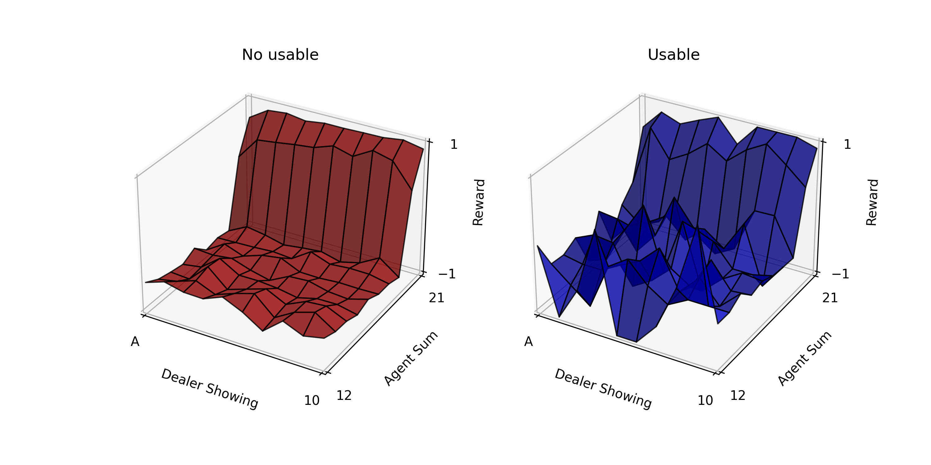
Fig.01 First-visit MC Prediction (10,000)
10,000번 시뮬레이션 진행한 결과를 이용해 First-visit MC Prediction을 수행한 모습

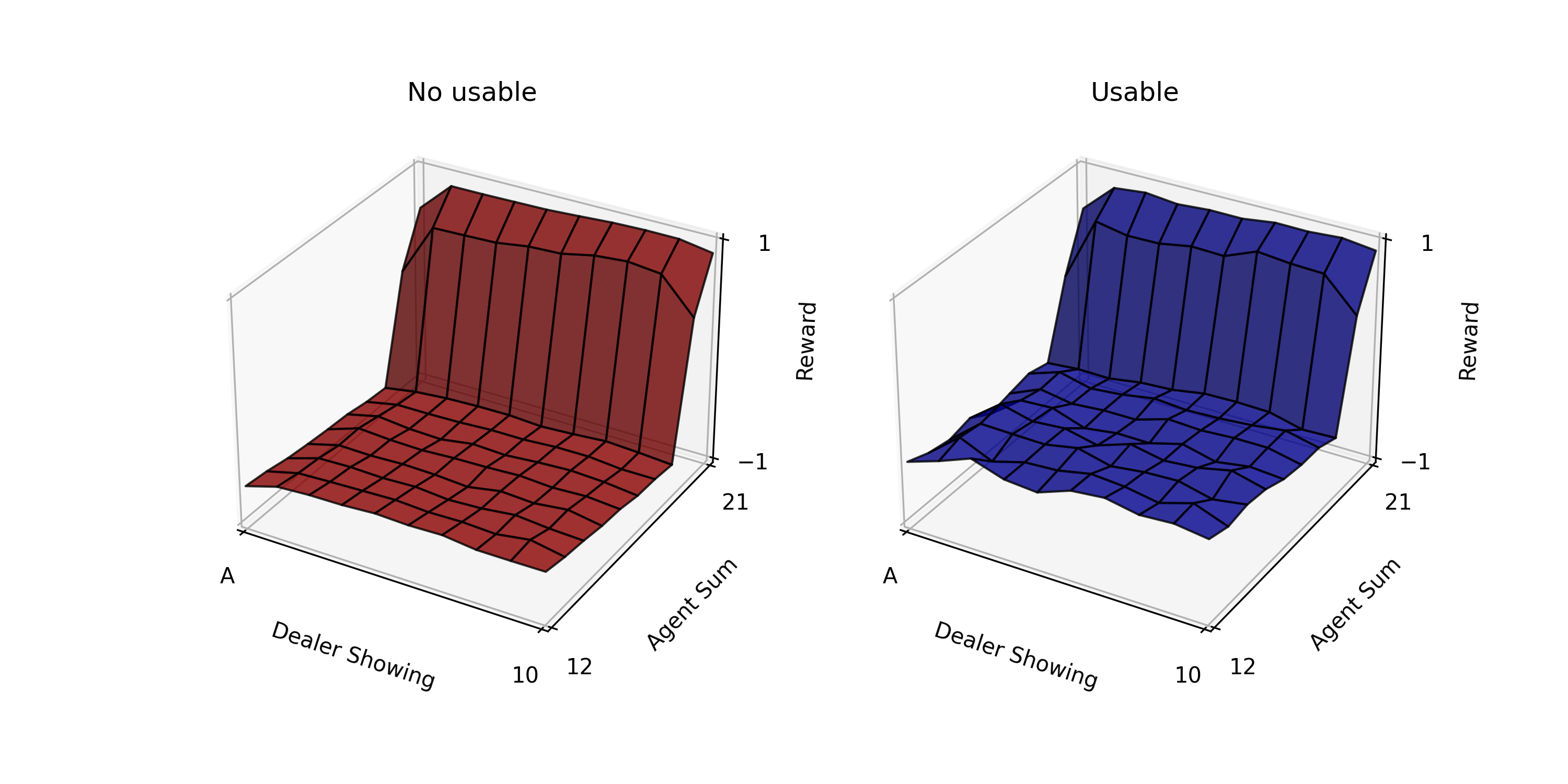
Fig.02 First-visit MC Prediction (500,000)
500,000번 시뮬레이션 진행한 결과를 이용해 First-visit MC Prediction을 수행한 모습

Fig.01을 보면 usable ace가 있는 경우의 그래프(파란색)가 더 울퉁불퉁한 것을 볼 수 있다. 이는 usable ace가 있는 경우가 드물기 때문에 데이터가 없어 이렇게 된 것이다. 시뮬레이션 횟수를 10,000번에서 500,000번으로 늘리면(Fig.02) 그래프가 평탄해지는 것을 볼 수 있다.

$q_{π}$ 추정하기

만약 환경에 대한 모델(model)이 있다면, $v_{π}$ 만 있어도 새로운 정책을 만들 수 있다.^[10] 하지만 모델이 없다면 $v_{π}$ 만으로는 새로운 정책을 만들 수 없다. 그러나 행동-가치 함수 $q_{π}$ 가 있다면 모델이 없어도(model-free) 최적 정책을 추정할 수 있다.^[11]

$q_{π}$ 를 추정하는 방법은 $v_{π}$ 를 추정하는 방법과 거의 같다. 우선 방문했다(visit) 는 단어를 다시 정의하자. 한 에피소드 안에서, 상태 $s$ 에서 행동 $a$ 가 수행된 것을 상태-행동 쌍(state-action pair) $(s, a)$ 에 방문했다(visit) 고 표현하고, $(s, a)$ 에 처음 방문했을 때를 $(s, a)$ 에 최초방문했다(first-visit) 고 표현한다.

그렇다면 다음 두 가지 경우를 생각할 수 있다.

First-visit MC Prediction : 상태-행동 쌍 $(s, a)$ 에 최초방문(first-visit)했을 때 받는 Return들의 평균으로 $q_{π} (s, a)$ 를 추정하는 방법
Every-visit MC Prediction : 상태-행동 쌍 $(s, a)$ 에 방문(visit)했을 때 받는 Return들의 평균으로 $q_{π} (s, a)$ 를 추정하는 방법

두 방법 모두 최초방문 및 방문 횟수가 커질수록 참값( $q_{π} (s, a)$ )에 수렴하게 된다.

그런데 한 가지 문제가 있다. MC Prediction으로 $q_{π} (s, a)$ 를 학습(추정)하려면 상태-행동 쌍 $(s, a)$ 에 방문한 경험이 있어야 하는데, 사실 많은 수의 상태-행동 쌍은 한 번도 방문당하지 않았을 수 있다.^[12] 특히 결정론적 정책(deterministic policy)을 사용한다면 각 상태마다 항상 동일한 행동만 하므로 각 상태에서 다양한 상태-행동 쌍을 관측할 수 없게 된다. GPI의 Improvement 과정을 진행하려면 각 상태에서 여러 개의 행동 중 가장 큰 가치를 가지는 행동을 선택해야 하는데, 이렇게 되면 비교 대상이 없어지게 된다.

이 문제를 해결하려면 계속해서 탐색(exploration)을 해 주면 된다.^[13] 탐색을 유지하는 방법에는 여러 가지가 있지만, 그 중 가장 유명한 두 가지를 소개하면 다음과 같다.

Exploring Starts : 모든 가능한 상태-행동 쌍 $(s, a)$ 에 대해, 각 에피소드가 이들 중 랜덤한 하나로 시작하게 하는 방법. 이렇게 하면 각 에피소드가 시작될 때 반드시 탐색(exploration)을 하게 된다. 에피소드 개수가 충분히 많으면 모든 상태-행동 쌍에 최소 한 번씩은 방문할 수 있게 된다. 그러나 이 방법은 실제 환경과 상호작용하며 학습하는 상황에서는 적용하기 어렵다는 단점이 있다.
확률적 정책(stochastic policy) 사용하기 : 결정론적 정책이더라도 확률적 정책으로 바꾸고, 각 상태의 모든 행동들에게 0이 아닌 확률을 부여하는 방법.

MC Prediction의 장점

MC Prediction은 DP에서 보았던, 주어진 정책 $π$ 에 대한 가치 함수를 계산하는 DP Policy Evaluation과 유사하다. 이때, MC Prediction은 DP Policy Evaluation에 비해 다음과 같은 장점을 가진다.

MC Prediction은 실제 경험과 시뮬레이션 결과로부터 학습이 가능하다. 하지만 DP Policy Evaluation은 경험으로부터 배우지 못하고, 반드시 환경에 대한 모든 정보를 알고 있을 때만 사용할 수 있다.
MC Prediction의 계산 난이도는 DP Policy Evaluation에 비해 아주 낮다. 여기서 말하는 계산 난이도는 알고리즘 시행 중의 난이도 뿐만 아니라 알고리즘을 사용하기 위한 전처리 계산의 난이도도 모두 포함한다. 예를 들어, 위 블랙잭 문제에서 DP Policy Evaluation을 사용하려면 우선 Dynamics Function $p$ 를 계산해야 한다. 그런데 $p$ 를 계산하는 일이 결코 만만하지 않다. 가령, $p (s^{'}, r = 1 ∥ s = (14, 10,$ False $), a =$ stick $)$ 은 얼마일까?^[14] DP Policy Evaluation을 사용하려면 DP Policy Evaluation 사용 전에 이런 값들을 모두 계산해 놓아야 한다. 그러나 MC Prediction을 쓰면 이런 계산을 할 필요가 없다.
MC Prediction에서 각 상태에 대한 가치 추정값은 각각 독립적이다. MC Prediction에서 한 상태의 가치 추정값은 DP Policy Evaluation에서처럼 다른 상태의 가치 추정값으로부터 만들어지지 않는다. 즉 MC Prediction은 Bootstrapping 하지 않는다. 이 덕분에 MC Prediction에서는 한 상태 또는 전체 상태의 부분집합에만 대해 가치를 추정할 수 있다. 반면 DP Policy Evaluation에서는 반드시 전체 상태에 대해 가치를 추정해야 한다.

MC Control(Monte Carlo Control)

GPI의 아이디어를 이용해 MC Method로 최적 정책을 추정(학습)하는 것을 MC Control(Monte Carlo Control)이라 한다.

MC Policy Iteration(Monte Carlo Policy Iteration)

MC Policy Iteration(Monte Carlo Policy Iteration)은 DP의 Policy Iteration을 MC Method 버전으로 바꾼 것이다.

먼저 논의를 쉽게 만드는 두 가지 가정을 해 보자.

가정 1. 관찰할 수 있는 에피소드의 개수는 무한개이다.
가정 2. 모든 에피소드에는 Exploring Starts가 적용되었다.

이제 GPI를 적용해 보자.

Evaluation 과정 : MC Prediction을 통해 정책 $π_{k}$ 로부터 행동-가치 함수 $q_{π_{k}}$ 를 추정한다. 가정 1, 2에 의해, 정확한 $q_{π_{k}}$ 을 구할 수 있다.
Improvement 과정 : $q_{π_{k}}$ 에 대해 탐욕적인(greedy) 정책을 만들어, 정책 $π_{k}$ 를 $π_{k + 1}$ 로 업데이트한다.^[15] Policy Improvement Theorem에 의해, $π_{k + 1}$ 은 $π_{k}$ 보다 항상 같거나 좋은 정책이 된다.

증명

현재 정책 $π_{k}$ 을 업데이트하여 정책 $π_{k + 1}$ 을 얻었다 해 보자. 이때,

\begin{aligned} q_{π_{k}} (s, π_{k + 1} (s)) & = q_{π_{k}} (s, \underset{a}{\arg \max} q_{π_{k}} (s, a)) \\ = max_{a} q_{π_{k}} (s, a) \\ \geq q_{π_{k}} (s, π_{k} (s)) \\ \geq v_{π_{k}} (s) \end{aligned}

가 성립한다. 따라서, Policy Improvement Theorem에 의해 $π_{k + 1} \geq π_{k}$ 이다(= $v_{π_{k + 1}} (s) \geq v_{π_{k}} (s)$ ).

이렇게 두 과정을 번갈아가며 진행하면, 환경에 대한 어떠한 배경 지식 없이도 최적 정책을 찾을 수 있다. 이때 Evaluation 과정과 Improvement 과정은 에피소드 단위로 진행된다(episode-by-episode). 각 에피소드가 끝나면, 관측된 Return을 이용해 가치 함수를 계산하고(Evaluation 과정), 해당 에피소드에서 방문한 모든 상태들에서의 정책이 업데이트된다(Improvement 과정). 그리고 다음 에피소드에 다시 Evaluation 과정과 Improvement 과정을 적용한다.

Monte Carlo ES(Monte Carlo with Exploring Starts)

하지만 위에 한 두 가정이 거슬란다. 위 두 가정은 MC Policy Iteration이 확실히 수렴하게 하기 위해 도입한 가정이었는데(조금 더 정확하게는, Evaluation 과정이 확실히 수렴하게 하기 위한 가정이었는데), 현실적이지 않다.

우선 가정 1, "관찰할 수 있는 에피소드의 개수는 무한개이다"를 없애보자. 가정 1을 없애는 방법은 두 가지가 있다.

추정의 정도(level of approximation)의 상한을 정하는 방법 : 상태-행동 쌍 $(s, a)$ 에 대해, 최신 가치 추정값과 옛 가치 추정값 사이의 차 $∥ q_{π_{k + 1}} (s, a) - q_{π_{k}} (s, a) ∥$ 의 최댓값이 일정 값( $θ$ )^[16] 이하로 떨어지면 멈춘다. 이 방법은 DP에서도 살펴본 방법이다. 그러나 이 방법을 실전에서 쓰려면 작은 문제에서도 엄청 많은 수의 에피소드가 있어야 한다는 단점이 있다.
Evaluation 과정을 다 마치지 않고 Improvement 과정으로 넘어가는 방법 : DP의 Value Iteration와 유사한 방법이다. 이렇게 하면 매 Evaluation 단계마다 가치 함수는 $q_{π_{k}}$ 에 다가가기는 하지만, 참값에 수렴할 때까지 하진 않는다. 보통은 이 방법을 많이 사용한다.

이렇게 가정 1을 없앤 (가정 2(모든 에피소드에는 Exploring Starts가 적용되었다)는 남아 있는) MC Policy Iteration을 Monte Carlo ES(Monte Carlo with Exploring Starts)라 한다. Monte Carlo ES를 의사 코드로 나타내면 다음과 같다.

Pseudo Code : Monte Carlo ES(Monte Carlo with Exploring Starts)

1. 초기화

모든 $s \in S$ 에 대해, $π (s)$ 를 임의의 행동 $a \in A$ 로 초기화

모든 $s \in S$ , $a \in A$ 에 대해, $Q (s, a)$ 을 임의의 실수로 초기화

모든 $s \in S$ , $a \in A$ 에 대해, Returns( $s$ , $a$ ) = [] (빈 리스트)로 초기화

2. Policy Iteration

Loop forever (for each episode):

# Exploring Start

$S_{0} \in S$ , $A_{0} \in A (S_{0})$ 를 랜덤으로 선택 # 단, 상태-행동 쌍 $(S_{0}, A_{0})$ 가 발생할 확률은 모두 0보다 커야 한다.

$(S_{0}, A_{0})$ 에서부터 $π$ 를 따라 에피소드 생성 : $S_{0}, A_{0}, R_{1}, S_{1}, A_{1}, R_{2}, \dots, S_{T - 1}, A_{T - 1}, R_{T}$

$G \leftarrow 0$

Loop for each step of episode, $t = T - 1, T - 2, \dots, 0$ :

$G \leftarrow γ G + R_{t + 1}$

If not $(S_{t}, A_{t})$ appears in $S_{0}, A_{0}, S_{1}, A_{1}, \dots, S_{t - 1}, A_{t - 1}$ :

Returns( $S_{t}, A_{t}$ ).append( $G$ )

$Q (S_{t}, A_{t}) \leftarrow$ average(Returns( $S_{t}, A_{t}$ ))

# Improvement 과정

$π (S_{t}) \leftarrow \underset{a}{\arg \max} Q (S_{t}, a)$

GPI에서 보았듯이 가치 함수와 정책이 모두 최적값에 도착했을 때 위 과정은 안정화된다. 따라서 Monte Carlo ES는 차(次)적 정책(suboptimal policy)로 빠지지 않고, 최적 정책으로 수렴하게 된다.^[17]

구현하기

Monte Carlo ES를 이용해 블랙잭 게임에서 최적 정책을 찾아 보자.

Code : Monte Carlo ES (First-visit MC Control)

python

import numpy as np
import matplotlib.pyplot as plt
from abc import *

def parseState(state):
    if state is None:
        return None
    elif state == -1:
        return (-1, -1, False)
    is_usable = True if (state // 100) == 1 else False
    agent_sum = (state % 100) // 10 + 12
    dealer_showing = state % 10 + 1
    return (agent_sum, dealer_showing, is_usable)

class Env:
    def __init__(self):
        self.deck = None
        self.agent_cards = None
        self.dealer_cards = None
    
    def _pop(self, target_card=None):
        if target_card is not None:
            pos = np.where(self.deck == target_card)[0][0]
            self.deck[-1], self.deck[pos] = self.deck[pos], self.deck[-1]
            
        card = self.deck[-1]
        self.deck = self.deck[0:-1]
        return card
    
    def _getCardScore(self, card):
        num = card % 13
        if num in [10, 11, 12]: # J, Q, K
            return 10
        else:
            return num + 1
    
    def _getCardsScore(self, cards):
        ace_count = 0
        total_score = 0
        for card in cards:
            score = self._getCardScore(card)
            total_score += score
            if score == 1:
                ace_count += 1
        
        is_usable = False
        if ace_count > 0 and total_score + 10 <= 21:
            ace_count -= 1
            total_score += 10
            is_usable = True
        
        return total_score, is_usable
    
    def _getRandomCardByScore(self, score):
        card = None
    
        if score == 10:
            card = np.random.choice([(x + 13 * i) for i in range(4) for x in [9, 10, 11, 12] if (x + 13 * i) in self.deck])
        else:
            card = np.random.choice([(score - 1 + 13 * i) for i in range(4) if (score - 1 + 13 * i) in self.deck])
            
        return card
    
    def _dealer_playing(self):
        while self._getCardsScore(self.dealer_cards)[0] < 17:
            self.dealer_cards.append(self._pop())
    
    def _getState(self):
        agent_sum, is_usable = self._getCardsScore(self.agent_cards)
        dealer_showing = self._getCardScore(self.dealer_cards[0])
        
        if agent_sum in range(12, 22) and dealer_showing in range(1, 11):
            return (1 if is_usable else 0) * 100 + (agent_sum - 12) * 10 + (dealer_showing - 1)
        else:
            return -1
    
    def newGame(self, s0=None):
        self.deck = np.arange(52, dtype=int)
        np.random.shuffle(self.deck)
        
        if s0 is not None:
            self.agent_cards = []
            self.dealer_cards = []
        
            agent_sum, dealer_showing, is_usable = parseState(s0)

            # dealer_cards[0]
            self.dealer_cards.append(self._pop(self._getRandomCardByScore(dealer_showing)))

            # dealer_cards[1]
            self.dealer_cards.append(self._pop())

            if is_usable:
                # agent_cards[0]
                self.agent_cards.append(self._pop(self._getRandomCardByScore(1)))

                # agent_cards[1]
                self.agent_cards.append(self._pop(self._getRandomCardByScore(agent_sum - 11)))
            else:
                score1, score2 = 0, 0
                while not (1 <= score1 <= 10 and 1 <= score2 <= 10):
                    score1 = np.random.choice(range(1, 11))
                    score2 = agent_sum - score1

                # agent_cards[0]
                self.agent_cards.append(self._pop(self._getRandomCardByScore(score1)))

                # agent_cards[1]
                self.agent_cards.append(self._pop(self._getRandomCardByScore(score2)))
        else:
            self.agent_cards = [self._pop() for x in range(2)]
            self.dealer_cards = [self._pop() for x in range(2)]
        
        return 0, self._getState(), 0
                
    def interact(self, action):
        if action == 0: # hit
            self.agent_cards.append(self._pop())
            if self._getCardsScore(self.agent_cards)[0] > 21: # agent bust
                return 1, self._getState(), -1
            else:
                return 0, self._getState(), 0
        else: # stick
            self._dealer_playing()
            agent_score = self._getCardsScore(self.agent_cards)[0]
            dealer_score = self._getCardsScore(self.dealer_cards)[0]
            
            if dealer_score > 21: # dealer bust
                return 1, self._getState(), 1
            else:
                if agent_score > dealer_score:
                    return 1, self._getState(), 1
                elif agent_score < dealer_score:
                    return 1, self._getState(), -1
                else:
                    return 1, self._getState(), 0

class Agent:
    def __init__(self, gamma=1):
        self.gamma = gamma
        self.policy = np.full(shape=(200, 2), fill_value=0.5, dtype=float)

    def action(self, state):
        if state == -1:
            return 0 # hit
        else:
            return np.random.choice([0, 1], p=self.policy[state])

class Trainer(metaclass=ABCMeta):
    def __init__(self, agent, env):
        self.agent = agent
        self.env = env
        
        self.initPolicy()
        
    def _decideActionByPolicy(self, policy, state):
        if state == -1:
            return 0 # hit
        else:
            return np.random.choice([0, 1], p=policy[state])
    
    def _simulate(self, policy, s0a0=None):
        R = []
        S = []
        A = []
        
        if s0a0 is not None:
            s0, a0 = s0a0
            
            status, state, reward = self.env.newGame(s0)
            reward = None
            
            R.append(reward)
            S.append(s0)
            A.append(a0)
            
            status, state, reward = self.env.interact(a0)
        else:
            status, state, reward = self.env.newGame()
            reward = None
            
        while status == 0:
            R.append(reward)
            S.append(state)

            action = self._decideActionByPolicy(policy=policy, state=state)
            A.append(action)
            status, state, reward = self.env.interact(action)

        R.append(reward)
        S.append(state)
        A.append(None)
        
        return R, S, A
    
    def initPolicy(self):
        pass
    
    @abstractmethod
    def train(self, trials):
        pass
                
    def test(self, trials):
        Returns = []
        for i in range(trials):
            R, S, A = self._simulate(policy=self.agent.policy)
            Returns.append(sum([x for x in R if x is not None]))

        print(f"Test Result({trials}) : {'%.2f' % (np.average(Returns))}")
    
    def drawPolicy(self):
        def getColor(state):
            argmax = np.where(self.agent.policy[state] == self.agent.policy[state].max())[0]
            if len(argmax) == 2: # both
                return 'yellow'
            else:
                if argmax[0] == 0: # hit
                    return 'green'
                else: # stick
                    return 'red'
        
        fig = plt.figure(figsize=(10, 5))
        subplots = [fig.add_subplot(1, 2, 1), fig.add_subplot(1, 2, 2)]
        
        # No usable
        x = [i for i in range(10) for j in range(10)] # dealer showing
        y = [j for i in range(10) for j in range(10)] # agent sum
        c = [getColor(y[i] * 10 + x[i]) for i in range(100)]
        subplots[0].scatter(x, y, c=c)
        subplots[0].set_title("No usable")
        
        # Usable
        x = [i for i in range(10) for j in range(10)] # dealer showing
        y = [j for i in range(10) for j in range(10)] # agent sum
        c = [getColor(100 + y[i] * 10 + x[i]) for i in range(100)]
        subplots[1].scatter(x, y, c=c)
        subplots[1].set_title("Usable")
        
        for subplot in subplots:
            subplot.set_xlim(0, 9)
            subplot.set_xticks([i for i in range(10)])
            subplot.set_xticklabels(['A'] + [str(i) for i in range(2, 11)])
            subplot.set_xlabel("Dealer Showing")
            subplot.set_ylim(0, 9)
            subplot.set_yticks([i for i in range(10)])
            subplot.set_yticklabels([str(i) for i in range(12, 22)])
            subplot.set_ylabel("Agent Sum")
        
        plt.show()

class MonteCarloESTrainer(Trainer):
    def initPolicy(self):
        for state in range(200):
            agent_sum, dealer_showing, is_usable = parseState(state)
            if agent_sum in [20, 21]:
                self.agent.policy[state][0] = 0 # hit
                self.agent.policy[state][1] = 1 # stick
            else:
                self.agent.policy[state][0] = 1 # hit
                self.agent.policy[state][1] = 0 # stick
        
    def train(self, trials):
        Q = np.zeros((200, 2), dtype=float)
        Returns = [[[] for a in range(2)] for s in range(200)]
        
        for trial in range(trials):
            s0 = np.random.choice([x for x in range(200) if not ((x // 100) == 0 and (x % 100) // 10 + 12 == 21)]) # remove the case that agent_sum = 21 and is_usable = False
            a0 = np.random.choice([0, 1]) # 0 : hit, 1 : stick
            
            R, S, A = self._simulate(policy=self.agent.policy, s0a0=(s0, a0))
            
            T = len(R)
            G = 0
            for t in reversed(range(T - 1)):
                G = self.agent.gamma * G + R[t + 1]
                
                if S[t] == -1:
                    continue
                else:
                    is_first_visit = True
                    for i in range(t):
                        if S[t] == S[i] and A[t] == A[i]:
                            is_first_visit = False
                            break
                    
                    if is_first_visit:
                        Returns[S[t]][A[t]].append(G)
                        Q[S[t]][A[t]] = np.average(Returns[S[t]][A[t]])
                        
                        # Improvement 과정
                        self.agent.policy[S[t]][0] = 1 if Q[S[t]][0] > Q[S[t]][1] else 0
                        self.agent.policy[S[t]][1] = 1 if Q[S[t]][0] <= Q[S[t]][1] else 0

if __name__ == "__main__":
    env = Env()
    agent = Agent()
    trainer = MonteCarloESTrainer(agent, env)

    print("Before Training...")
    trainer.test(trials=10000)
    trainer.drawPolicy()
    
    trainer.train(500000)
    
    print("After Training...")
    trainer.test(trials=10000)
    trainer.drawPolicy()

1
2
3
4
5
6
7
8
9
10
11
12
13
14
15
16
17
18
19
20
21
22
23
24
25
26
27
28
29
30
31
32
33
34
35
36
37
38
39
40
41
42
43
44
45
46
47
48
49
50
51
52
53
54
55
56
57
58
59
60
61
62
63
64
65
66
67
68
69
70
71
72
73
74
75
76
77
78
79
80
81
82
83
84
85
86
87
88
89
90
91
92
93
94
95
96
97
98
99
100
101
102
103
104
105
106
107
108
109
110
111
112
113
114
115
116
117
118
119
120
121
122
123
124
125
126
127
128
129
130
131
132
133
134
135
136
137
138
139
140
141
142
143
144
145
146
147
148
149
150
151
152
153
154
155
156
157
158
159
160
161
162
163
164
165
166
167
168
169
170
171
172
173
174
175
176
177
178
179
180
181
182
183
184
185
186
187
188
189
190
191
192
193
194
195
196
197
198
199
200
201
202
203
204
205
206
207
208
209
210
211
212
213
214
215
216
217
218
219
220
221
222
223
224
225
226
227
228
229
230
231
232
233
234
235
236
237
238
239
240
241
242
243
244
245
246
247
248
249
250
251
252
253
254
255
256
257
258
259
260
261
262
263
264
265
266
267
268
269
270
271
272
273
274
275
276
277
278
279
280
281
282
283
284
285
286
287
288
289
290
291
292
293
294
295
296
297
298
299
300
301
302
303
304
305
306
307

코드 설명

line 5 ~ 13 : parseState()
- state가 무슨 의미인지 해석하는 함수
- state를 입력값으로 받아 agent_sum, dealer_showing, is_usable을 반환
line 15 ~ 136 : 환경(Environment)을 나타내는 클래스
- line 21 ~ 28 : Env._pop()
  - target_card 파라미터가 주어지지 않은 경우, 덱에서 첫 번째 카드를 뽑는다.
  - target_card 파라미터가 주어진 경우, 덱에서 target_card를 뽑는다.
- line 30 ~ 35 : Env._getCardScore()
  - card의 점수를 반환하는 메서드
  - Ace 카드는 1점으로 계산
- line 37 ~ 52 : Env._getCardsScore()
  - cards 안 카드들의 점수의 합 total_score와 usable ace가 있는지의 여부 is_usable을 조사해서 반환하는 메서드
- line 54 ~ 62 : Env._getRandomCardByScore()
  - 점수가 score인, 덱에 존재하는 카드 중 무작위로 하나를 반환하는 메서드
- line 64 ~ 66 : Env._dealer_playing()
  - 딜러가 정해진 규칙에 따라 플레이하는 메서드
- line 68 ~ 75 : Env._getState()
  - 현재 상태(state)를 반환하는 메서드
- line 77 ~ 114 : Env.newGame()
  - 에이전트와 딜러의 패를 초기화하는 메서드
  - 현재 게임 진행 상태(0: 게임 진행 중, 1: 게임 오버), 상태(Env._getState() 메서드 이용), 보상(0) 반환
  - s0 파라미터가 주어진 경우, 초기 상태 s0에 해당하도록 에이전트와 딜러의 패를 만든다(Env._getRandomCardByScore() 메서드 이용).
  - s0 파라미터가 주어지지 않은 경우, 에이전트와 딜러의 패를 무작위적으로 만든다.
- line 116 ~ 136 : Env.interact()
  - 게임을 진행하는 메서드
  - 에이전트의 행동 action(0: hit, 1: stick)을 입력받아 그 결과(현재 게임 진행 상태, 상태, 보상)를 반환
line 138 ~ 147 : 에이전트를 나타내는 클래스
- line 139 ~ 141 : Agent.__init__() 메서드
  - $γ$ , self.policy 초기화
- line 143 ~ 147 : Agent.action() 메서드
  - self.policy에 따라, 파라미터로 입력받은 상태 state에서의 행동을 반환
  - 만약 state가 -1이면(= 현재 에이전트의 패의 점수가 11 이하면) 무조건 hit을 선택
line 149 ~ 249 : 학습을 진행하는 Trainer 클래스
- line 150 ~ 154 : Trainer.__init__()
  - 에이전트 agent, 환경 env 등록
  - 에이전트의 정책 초기화(self.initPolicy())
- line 156 ~ 160 : Trainer._decideActionByPolicy()
  - 상태 state에서 정책 policy를 따를 때의 행동을 반환
  - 만약 state가 -1이면(= 현재 에이전트의 패의 점수가 11 이하면) 무조건 hit을 선택
  - Agent.action()과 유사
- line 162 ~ 194 : Trainer._simulate()
  - 정책 policy를 따라 시뮬레이션을 진행하는 메서드
  - 각 시간 단계별 보상, 상태, 행동을 담고 있는 리스트 R, S, A 반환
  - s0a0 파라미터가 주어진 경우, 초기 상태 s0에서 행동 a0를 수행한 후 정책 policy를 따라 시뮬레이션을 진행한다.
  - s0a0 파라미터가 주어지지 않은 경우, 정책 policy를 따라 시뮬레이션을 진행한다.
- line 196 ~ 197 : Trainer.initPolicy()
  - 에이전트의 정책을 초기화하는 메서드
  - Agent.__init__()에서 초기화를 이미 한 번 하기 때문에, 기본적으론 아무 동작도 하지 않음(필요하다면 override해 사용)
- line 199 ~ 201 : Trainer.train()
  - 학습을 진행하는 (추상) 메서드
- line 203 ~ 209 : Trainer.test()
  - 현재 에이전트의 정책을 사용하여 trials 번의 시뮬레이션을 수행해, 받는 보상들의 평균을 계산하는 메서드
- line 211 ~ 249 : Trainer.drawPolicy()
  - 현재 에이전트의 정책을 시각화한 그래프를 출력하는 메서드
  - 초록 점은 hit, 빨간 점은 stick, 노란 점은 hit과 stick 둘 중에 아무거나 선택해도 됨을 의미한다.
line 251 ~ 292 : Monte Carlo ES를 수행하는 Trainer 클래스
- line 252 ~ 260 : MonteCarloESTrainer.initPolicy() 메서드
  - 에이전트의 정책을 초기화하는 메서드(override)
  - agent_sum이 20 또는 21인 경우 stick, 나머지의 경우 hit을 사용하는 정책
- line 262 ~ 292 : MonteCarloESTrainer.train() 메서드
  - 학습을 진행하는 메서드
line 294 ~ 307 : main
- 에이전트와 환경을 만들어 성능평가를 하고, 500,000번의 시행을 통해 학습을 한 후 다시 성능평가를 진행

Fig.03 Monte Carlo ES를 이용한 First-visit MC Control
500,000번 시뮬레이션 진행한 결과를 이용해 Monte Carlo ES로 First-visit MC Control을 수행

Fig.03은 위 코드의 실행 결과를 보여준다. 학습 전에는 보상들의 평균으로 -0.36을 얻다가 학습 후에는 -0.04를 얻는 것을 볼 수 있다.

On-policy MC Control without ES(On-policy Monte Carlo Control without Exploring Starts)

가정 2, "모든 에피소드에는 Exploring Starts가 적용되었다"를 없애는 것은 가정 1을 없애는 것보다 조금 더 복잡하다.

MC Control은 크게 On-policy MC Control과 Off-policy MC Control, 이렇게 두 종류로 분류할 수 있다. On-policy MC Control에서는 학습을 위한 데이터를 만들 때 사용하는 정책과 평가(evaluate), 개선(improve)이 이루어지는 정책이 서로 같다. 즉 데이터를 만들 때 사용한 정책을 바로 평가, 개선하는 것이다. 예를 들어 위 문단에서 살펴본 Monte Carlo ES는 On-policy MC Control이다. 하지만 Off-policy MC Control에서는 학습을 위한 데이터를 만들 때 사용하는 정책과 평가, 개선이 이루어지는 정책이 서로 다르다. On-policy MC Control과 Off-policy MC Control에 대한 더 자세한 얘기는 아래 문단에서 계속하겠다.

우선 On-policy MC Control에서 가정 2, "모든 에피소드에는 Exploring Starts가 적용되었다"를 제거해보자. 이를 위해선 먼저 *부드럽다(soft)*는 용어를 정의해야 한다. 정책 $π$ 가 모든 상태 $s \in S$ 와 모든 행동 $a \in A (s)$ 에 대해 $π (a ∥ s) > 0$ 이 성립하면, 해당 정책 $π$ 를 부드럽다고 한다.^[18]

부드러운 정책의 예로 $ε$ -greedy policy가 있다. $ε$ -greedy policy는 다음과 같이 작동한다.

대부분의 경우에는( $1 - ε$ 의 확률로) 가장 큰 action value 추정값를 가진 행동을 선택한다.
간간히( $ε$ 의 확률로) 완전 무작위적인 행동을 선택한다.

이렇게 하면 모든 비탐욕적인(nongreedy) 행동은 $\frac{ε}{∥ A (s) ∥}$ 의 확률로 선택되고, 탐욕적인 행동은 $1 - ε + \frac{ε}{∥ A (s) ∥}$ 의 확률로 선택된다. 모든 가능한 $(s, a)$ 쌍에 대해 $π (a ∥ s) > 0$ 이 성립되므로 $ε$ -greedy policy는 부드러운 정책이다.

$ε$ -greedy policy를 확장하면 $ε$ -soft policy를 만들 수 있다. 적당한 $ε > 0$ 에 대해, 모든 가능한 $(s, a)$ 쌍에서 $π (a ∥ s) \geq \frac{ε}{∥ A (s) ∥}$ 이 성립하면 정책 $π$ 를 $ε$ -soft policy라 한다. 즉 말하자면 $ε$ -greedy policy는 $ε$ -soft policy 중 가장 탐욕적인 정책이다.

$ε$ -soft policy를 이용하면 On-policy MC Control에서 가정 2를 제거할 수 있다. 핵심 아이디어는 GPI를 유지하되, Improvement 과정에서 현재 정책을 완전한 탐욕 정책(greedy policy)이 되게 업데이트하지 않고, 적당히 그 근처( $ε$ -greedy policy)로 업데이트하는 것이다. Policy Improvement Theorem에 의해, 실제 행동-가치 함수 $q_{π}$ 에 대한 모든 $ε$ -greedy policy은 어떠한 $ε$ -soft policy보다도 좋거나 낫다.

증명

$ε$ -soft policy $π$ 와 $q_{π}$ 에 대한 $ε$ -greedy policy $π^{'}$ 가 있다고 해 보자. 모든 $s \in S$ 에 대해,

\begin{aligned} q_{π} (s, π^{'} (s)) & = \sum_{a} π^{'} (a | s) q_{π} (s, a) \\ = \frac{ε}{| A (s) |} \sum_{a} q_{π} (s, a) + (1 - ε) max_{a} q_{π} (s, a) \\ \geq \frac{ε}{| A (s) |} \sum_{a} q_{π} (s, a) + (1 - ε) \sum_{a} \frac{π (a | s) - \frac{ε}{| A (s) |}}{1 - ε} q_{π} (s, a) \\ = \frac{ε}{| A (s) |} \sum_{a} q_{π} (s, a) - \frac{ε}{| A (s) |} \sum_{a} q_{π} (s, a) + \sum_{a} π (a | s) q_{π} (s, a) \\ = v_{π} (s) \end{aligned}

가 된다. 따라서, Policy Improvement Theorem에 의해 $π^{'} \geq π$ 이다(= $v_{π^{'}} (s) \geq v_{π} (s)$ ).

이 방법으로 얻는 정책은 100% 완벽한 최적 정책이 아닌, $ε$ -soft policy 중 가장 좋은 정책이긴 하지만, 어쨌든 exploring starts를 제거할 수 있다. 이 방법을 의사 코드로 나타내면 다음과 같다.

Pseudo Code : On-policy first-visit MC control( $ε$ -soft policy 사용)

1. 초기화

임의의 $ϵ$ -soft policy로 정책 $π$ 초기화

모든 $s \in S$ , $a \in A$ 에 대해, $Q (s, a)$ 을 임의의 실수로 초기화

모든 $s \in S$ , $a \in A$ 에 대해, Returns( $s$ , $a$ ) = [] (빈 리스트)로 초기화

2. On-policy first visit MC Control

Loop forever (for each episode):

$π$ 를 따라 에피소드 생성 : $S_{0}, A_{0}, R_{1}, S_{1}, A_{1}, R_{2}, \dots, S_{T - 1}, A_{T - 1}, R_{T}$

$G \leftarrow 0$

Loop for each step of episode, $t = T - 1, T - 2, \dots, 0$ :

$G \leftarrow γ G + R_{t + 1}$

If not $(S_{t}, A_{t})$ appears in $S_{0}, A_{0}, S_{1}, A_{1}, \dots, S_{t - 1}, A_{t - 1}$ :

Returns( $S_{t}, A_{t}$ ).append( $G$ )

$Q (S_{t}, A_{t}) \leftarrow$ average(Returns( $S_{t}, A_{t}$ ))

# Improvement 과정

$A^{\*} \leftarrow \underset{a}{\arg \max} Q (S_{t}, a)$ # 만약 $Q (S_{t}, a)$ 를 최대로 만드는 $a$ 가 여러 개이면 그 중 랜덤하게 고른다.

모든 $a \in A (S_{t})$ 에 대해,

$π (a | S_{t}) \leftarrow {\begin{cases} 1 - ε + \frac{ε}{| A (S_{t}) |} & if a = A^{*} \\ \frac{ε}{| A (S_{t}) |} & if a \neq A^{*} \end{cases}$

구현하기

$ε$ -soft policy를 사용하는 On-policy first-visit MC control을 이용해 블랙잭 게임에서 최적 정책을 찾아보자.

Code : On-policy first-visit MC control(

ε

-soft policy 사용)

python

import numpy as np
import matplotlib.pyplot as plt
from abc import *

def parseState(state):
    if state is None:
        return None
    elif state == -1:
        return (-1, -1, False)
    is_usable = True if (state // 100) == 1 else False
    agent_sum = (state % 100) // 10 + 12
    dealer_showing = state % 10 + 1
    return (agent_sum, dealer_showing, is_usable)

class Env:
    def __init__(self):
        self.deck = None
        self.agent_cards = None
        self.dealer_cards = None
    
    def _pop(self, target_card=None):
        if target_card is not None:
            pos = np.where(self.deck == target_card)[0][0]
            self.deck[-1], self.deck[pos] = self.deck[pos], self.deck[-1]
            
        card = self.deck[-1]
        self.deck = self.deck[0:-1]
        return card
    
    def _getCardScore(self, card):
        num = card % 13
        if num in [10, 11, 12]: # J, Q, K
            return 10
        else:
            return num + 1
    
    def _getCardsScore(self, cards):
        ace_count = 0
        total_score = 0
        for card in cards:
            score = self._getCardScore(card)
            total_score += score
            if score == 1:
                ace_count += 1
        
        is_usable = False
        if ace_count > 0 and total_score + 10 <= 21:
            ace_count -= 1
            total_score += 10
            is_usable = True
        
        return total_score, is_usable
    
    def _getRandomCardByScore(self, score):
        card = None
    
        if score == 10:
            card = np.random.choice([(x + 13 * i) for i in range(4) for x in [9, 10, 11, 12] if (x + 13 * i) in self.deck])
        else:
            card = np.random.choice([(score - 1 + 13 * i) for i in range(4) if (score - 1 + 13 * i) in self.deck])
            
        return card
    
    def _dealer_playing(self):
        while self._getCardsScore(self.dealer_cards)[0] < 17:
            self.dealer_cards.append(self._pop())
    
    def _getState(self):
        agent_sum, is_usable = self._getCardsScore(self.agent_cards)
        dealer_showing = self._getCardScore(self.dealer_cards[0])
        
        if agent_sum in range(12, 22) and dealer_showing in range(1, 11):
            return (1 if is_usable else 0) * 100 + (agent_sum - 12) * 10 + (dealer_showing - 1)
        else:
            return -1
    
    def newGame(self, s0=None):
        self.deck = np.arange(52, dtype=int)
        np.random.shuffle(self.deck)
        
        if s0 is not None:
            self.agent_cards = []
            self.dealer_cards = []
        
            agent_sum, dealer_showing, is_usable = parseState(s0)

            # dealer_cards[0]
            self.dealer_cards.append(self._pop(self._getRandomCardByScore(dealer_showing)))

            # dealer_cards[1]
            self.dealer_cards.append(self._pop())

            if is_usable:
                # agent_cards[0]
                self.agent_cards.append(self._pop(self._getRandomCardByScore(1)))

                # agent_cards[1]
                self.agent_cards.append(self._pop(self._getRandomCardByScore(agent_sum - 11)))
            else:
                score1, score2 = 0, 0
                while not (1 <= score1 <= 10 and 1 <= score2 <= 10):
                    score1 = np.random.choice(range(1, 11))
                    score2 = agent_sum - score1

                # agent_cards[0]
                self.agent_cards.append(self._pop(self._getRandomCardByScore(score1)))

                # agent_cards[1]
                self.agent_cards.append(self._pop(self._getRandomCardByScore(score2)))
        else:
            self.agent_cards = [self._pop() for x in range(2)]
            self.dealer_cards = [self._pop() for x in range(2)]
        
        return 0, self._getState(), 0
                
    def interact(self, action):
        if action == 0: # hit
            self.agent_cards.append(self._pop())
            if self._getCardsScore(self.agent_cards)[0] > 21: # agent bust
                return 1, self._getState(), -1
            else:
                return 0, self._getState(), 0
        else: # stick
            self._dealer_playing()
            agent_score = self._getCardsScore(self.agent_cards)[0]
            dealer_score = self._getCardsScore(self.dealer_cards)[0]
            
            if dealer_score > 21: # dealer bust
                return 1, self._getState(), 1
            else:
                if agent_score > dealer_score:
                    return 1, self._getState(), 1
                elif agent_score < dealer_score:
                    return 1, self._getState(), -1
                else:
                    return 1, self._getState(), 0

class Agent:
    def __init__(self, gamma=1):
        self.gamma = gamma
        self.policy = np.full(shape=(200, 2), fill_value=0.5, dtype=float)

    def action(self, state):
        if state == -1:
            return 0 # hit
        else:
            return np.random.choice([0, 1], p=self.policy[state])

class Trainer(metaclass=ABCMeta):
    def __init__(self, agent, env):
        self.agent = agent
        self.env = env
        
        self.initPolicy()
        
    def _decideActionByPolicy(self, policy, state):
        if state == -1:
            return 0 # hit
        else:
            return np.random.choice([0, 1], p=policy[state])
    
    def _simulate(self, policy, s0a0=None):
        R = []
        S = []
        A = []
        
        if s0a0 is not None:
            s0, a0 = s0a0
            
            status, state, reward = self.env.newGame(s0)
            reward = None
            
            R.append(reward)
            S.append(s0)
            A.append(a0)
            
            status, state, reward = self.env.interact(a0)
        else:
            status, state, reward = self.env.newGame()
            reward = None
            
        while status == 0:
            R.append(reward)
            S.append(state)

            action = self._decideActionByPolicy(policy=policy, state=state)
            A.append(action)
            status, state, reward = self.env.interact(action)

        R.append(reward)
        S.append(state)
        A.append(None)
        
        return R, S, A
    
    def initPolicy(self):
        pass
    
    @abstractmethod
    def train(self, trials):
        pass
                
    def test(self, trials):
        Returns = []
        for i in range(trials):
            R, S, A = self._simulate(policy=self.agent.policy)
            Returns.append(sum([x for x in R if x is not None]))

        print(f"Test Result({trials}) : {'%.2f' % (np.average(Returns))}")
    
    def drawPolicy(self):
        def getColor(state):
            argmax = np.where(self.agent.policy[state] == self.agent.policy[state].max())[0]
            if len(argmax) == 2: # both
                return 'yellow'
            else:
                if argmax[0] == 0: # hit
                    return 'green'
                else: # stick
                    return 'red'
        
        fig = plt.figure(figsize=(10, 5))
        subplots = [fig.add_subplot(1, 2, 1), fig.add_subplot(1, 2, 2)]
        
        # No usable
        x = [i for i in range(10) for j in range(10)] # dealer showing
        y = [j for i in range(10) for j in range(10)] # agent sum
        c = [getColor(y[i] * 10 + x[i]) for i in range(100)]
        subplots[0].scatter(x, y, c=c)
        subplots[0].set_title("No usable")
        
        # Usable
        x = [i for i in range(10) for j in range(10)] # dealer showing
        y = [j for i in range(10) for j in range(10)] # agent sum
        c = [getColor(100 + y[i] * 10 + x[i]) for i in range(100)]
        subplots[1].scatter(x, y, c=c)
        subplots[1].set_title("Usable")
        
        for subplot in subplots:
            subplot.set_xlim(0, 9)
            subplot.set_xticks([i for i in range(10)])
            subplot.set_xticklabels(['A'] + [str(i) for i in range(2, 11)])
            subplot.set_xlabel("Dealer Showing")
            subplot.set_ylim(0, 9)
            subplot.set_yticks([i for i in range(10)])
            subplot.set_yticklabels([str(i) for i in range(12, 22)])
            subplot.set_ylabel("Agent Sum")
        
        plt.show()

class OnPolicyEpsilonSoftTrainer(Trainer):
    def __init__(self, agent, env, epsilon):
        self.epsilon = epsilon
        super().__init__(agent, env)
        
    def initPolicy(self):
        self.agent.policy[:, 0] = np.random.uniform(low=self.epsilon, high=1 - self.epsilon, size=200)
        self.agent.policy[:, 1] = 1 - self.agent.policy[:, 0]
        
    def train(self, trials):
        self.initPolicy()
        
        Q = np.zeros((200, 2), dtype=float)
        Returns = [[[] for a in range(2)] for s in range(200)]
        
        for trial in range(trials):
            R, S, A = self._simulate(policy=self.agent.policy)
            
            T = len(R)
            G = 0
            for t in reversed(range(T - 1)):
                G = self.agent.gamma * G + R[t + 1]
                
                if S[t] == -1:
                    continue
                else:
                    is_first_visit = True
                    for i in range(t):
                        if S[t] == S[i] and A[t] == A[i]:
                            is_first_visit = False
                            break
                    
                    if is_first_visit:
                        Returns[S[t]][A[t]].append(G)
                        Q[S[t]][A[t]] = np.average(Returns[S[t]][A[t]])
                        
                        # Improvement 과정
                        A_star = np.random.choice(np.where(Q[S[t]] == Q[S[t]].max())[0])
                        self.agent.policy[S[t]][A_star] = 1 - self.epsilon + self.epsilon / 2
                        self.agent.policy[S[t]][1 - A_star] = self.epsilon / 2

if __name__ == "__main__":
    env = Env()
    agent = Agent()
    trainer = OnPolicyEpsilonSoftTrainer(agent, env, epsilon=0.2)

    print("Before Training...")
    trainer.test(trials=10000)
    trainer.drawPolicy()
    
    trainer.train(500000)
    
    print("After Training...")
    trainer.test(trials=10000)
    trainer.drawPolicy()

코드 설명

line 5 ~ 13 : parseState()
- state가 무슨 의미인지 해석하는 함수
- state를 입력값으로 받아 agent_sum, dealer_showing, is_usable을 반환
line 15 ~ 136 : 환경(Environment)을 나타내는 클래스
- line 21 ~ 28 : Env._pop()
  - target_card 파라미터가 주어지지 않은 경우, 덱에서 첫 번째 카드를 뽑는다.
  - target_card 파라미터가 주어진 경우, 덱에서 target_card를 뽑는다.
- line 30 ~ 35 : Env._getCardScore()
  - card의 점수를 반환하는 메서드
  - Ace 카드는 1점으로 계산
- line 37 ~ 52 : Env._getCardsScore()
  - cards 안 카드들의 점수의 합 total_score와 usable ace가 있는지의 여부 is_usable을 조사해서 반환하는 메서드
- line 54 ~ 62 : Env._getRandomCardByScore()
  - 점수가 score인, 덱에 존재하는 카드 중 무작위로 하나를 반환하는 메서드
- line 64 ~ 66 : Env._dealer_playing()
  - 딜러가 정해진 규칙에 따라 플레이하는 메서드
- line 68 ~ 75 : Env._getState()
  - 현재 상태(state)를 반환하는 메서드
- line 77 ~ 114 : Env.newGame()
  - 에이전트와 딜러의 패를 초기화하는 메서드
  - 현재 게임 진행 상태(0: 게임 진행 중, 1: 게임 오버), 상태(Env._getState() 메서드 이용), 보상(0) 반환
  - s0 파라미터가 주어진 경우, 초기 상태 s0에 해당하도록 에이전트와 딜러의 패를 만든다(Env._getRandomCardByScore() 메서드 이용).
  - s0 파라미터가 주어지지 않은 경우, 에이전트와 딜러의 패를 무작위적으로 만든다.
- line 116 ~ 136 : Env.interact()
  - 게임을 진행하는 메서드
  - 에이전트의 행동 action(0: hit, 1: stick)을 입력받아 그 결과(현재 게임 진행 상태, 상태, 보상)를 반환
line 138 ~ 147 : 에이전트를 나타내는 클래스
- line 139 ~ 141 : Agent.__init__() 메서드
  - $γ$ , self.policy 초기화
- line 143 ~ 147 : Agent.action() 메서드
  - self.policy에 따라, 파라미터로 입력받은 상태 state에서의 행동을 반환
  - 만약 state가 -1이면(= 현재 에이전트의 패의 점수가 11 이하면) 무조건 hit을 선택
line 149 ~ 249 : 학습을 진행하는 Trainer 클래스
- line 150 ~ 154 : Trainer.__init__()
  - 에이전트 agent, 환경 env 등록
  - 에이전트의 정책 초기화(self.initPolicy())
- line 156 ~ 160 : Trainer._decideActionByPolicy()
  - 상태 state에서 정책 policy를 따를 때의 행동을 반환
  - 만약 state가 -1이면(= 현재 에이전트의 패의 점수가 11 이하면) 무조건 hit을 선택
  - Agent.action()과 유사
- line 162 ~ 194 : Trainer._simulate()
  - 정책 policy를 따라 시뮬레이션을 진행하는 메서드
  - 각 시간 단계별 보상, 상태, 행동을 담고 있는 리스트 R, S, A 반환
  - s0a0 파라미터가 주어진 경우, 초기 상태 s0에서 행동 a0를 수행한 후 정책 policy를 따라 시뮬레이션을 진행한다.
  - s0a0 파라미터가 주어지지 않은 경우, 정책 policy를 따라 시뮬레이션을 진행한다.
- line 196 ~ 197 : Trainer.initPolicy()
  - 에이전트의 정책을 초기화하는 메서드
  - Agent.__init__()에서 초기화를 이미 한 번 하기 때문에, 기본적으론 아무 동작도 하지 않음(필요하다면 override해 사용)
- line 199 ~ 201 : Trainer.train()
  - 학습을 진행하는 (추상) 메서드
- line 203 ~ 209 : Trainer.test()
  - 현재 에이전트의 정책을 사용하여 trials 번의 시뮬레이션을 수행해, 받는 보상들의 평균을 계산하는 메서드
- line 211 ~ 249 : Trainer.drawPolicy()
  - 현재 에이전트의 정책을 시각화한 그래프를 출력하는 메서드
  - 초록 점은 hit, 빨간 점은 stick, 노란 점은 hit과 stick 둘 중에 아무거나 선택해도 됨을 의미한다.
line 251 ~ 290 : On-policy First-visit MC Control Trainer 클래스
- line 252 ~ 254 : OnPolicyEpsilonSoftTrainer.__init__()
  - $ε$ 값을 의미하는 epsilon을 입력받아 초기화한다.
- line 256 ~ 258 : OnPolicyEpsilonSoftTrainer.initPolicy()
  - 에이전트의 정책을 초기화하는 메서드(override)
  - 무작위로 초기화
- line 260 ~ 290 : OnPolicyEpsilonSoftTrainer.train() 메서드
  - 학습을 진행하는 메서드
line 292 ~ 305 : main
- 에이전트와 환경을 만들어 성능평가를 하고, 500,000번의 시행을 통해 학습을 한 후 다시 성능평가를 진행

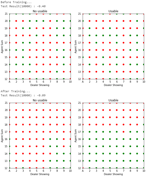
Fig.04 On-policy First-visit MC Control($\varepsilon$-soft policy 사용) — Fig.04 On-policy First-visit MC Control( $ε$ -soft policy 사용)
500,000번 시뮬레이션 진행한 결과를 이용해 On-policy First-visit MC Control을 수행

Fig.04는 위 코드의 실행 결과를 보여준다. 학습 전에는 보상들의 평균으로 -0.40을 얻다가 학습 후에는 -0.09를 얻는 것을 볼 수 있다.

Off-policy MC Method(Off-policy Monte Carlo Method)

최적 정책을 학습할 땐 딜레마를 마주하게 된다. 최적 정책을 찾기 위해선 최적이 아닌 행동을 해 탐색을 수행해야 한다. 위 문단에서 살펴본 On-policy MC Control은 정말 최적 정책을 찾은 것이 아니라, 최적과 가까운 정책(near-optimal policy)을 찾는, 사실상 타협을 한 것이다. 이보다 더 명확한 방법은 최적 정책이 되도록 학습하는 정책 하나와, 학습을 위한 데이터를 만들어내는 더 탐색적인(exploratory) 정책 하나, 이렇게 두 개의 정책을 분리해 사용하는 것이다. 이를 Off-policy MC Control이라 한다. 이때 학습이 이루어지는 정책을 목표 정책(target policy), 데이터를 생성하는 정책을 행동 정책(behavior policy) 이라 한다. Off-policy MC Control에서는 탐색용 정책이 따로 있기 때문에 Exploring Starts을 사용할 필요가 없다.

일반적으로 Off-policy MC Control이 On-policy MC Control보다 더 복잡하기에, 많은 경우 그냥 On-policy MC Control을 사용한다. 또한 Off-policy method에서는 다른 정책(행동 정책)으로 만든 데이터를 이용해 목표 정책을 학습시키기에 수렴 속도가 느리고 분산(variance)이 커진다는 단점이 있다. 하지만 Off-policy method는 더 범용적이고 더 강력하다는 장점이 있다. On-policy method는 Off-policy method에서 목표 정책과 행동 정책이 같은 특별 케이스라 이해할 수 있다.

Off-policy Prediction

Off-policy MC Control에 대해 알아보기에 앞서, 목표 정책 $π$ 와 행동 정책 $b \neq π$ 가 주어졌을 때 이로부터 목표 정책 $π$ 에 대한 가치 함수 $v_{π}$ 와 $q_{π}$ 를 추정하는 Off-policy Prediction에 대해 먼저 알아보자.

Off-policy Prediction을 위해서는 먼저 커버리지 가정(the assumption of coverage)과 Importance Sampling에 대해 알아야 한다.

우선 커버리지 가정부터 알아보자. 행동 정책 $b$ 로 만든 에피소드들을 이용해 목표 정책 $π$ 에 대한 가치 함수 $v_{π}$ 와 $q_{π}$ 를 추정하기 위해서는 $π$ 를 따를 때 선택되는 모든 행동들이 $b$ 를 따를 때에도, 항상은 아니더라도 간간히라도, 100% 선택되어야 한다. 이를 커버리지 가정(the assumption of coverage) 이라 한다.

커버리지 가정(The Assumption of Coverage)

Off-policy Prediction이 가능하려면, 반드시 다음이 성립해야 한다.

어떤 상태 $s$ 와 행동 $a$ 에 대해서 $π (a ∥ s) > 0$ 이면 반드시 $b (a ∥ s) > 0$ 이어야 한다.

커버리지 가정은 행동 정책 $b$ 가 반드시 확률적 정책(stochastic policy)이어야 함을^[19] 함축하고 있다. 그러나 목표 정책 $π$ 는 결정론적 정책(deterministic policy)이어도 상관없다.

이제 Importance Sampling에 대해 알아보자. Importance Sampling은 한 분포(distribution)의 기댓값을 다른 분포로부터의 샘플을 이용해 추정하는 테크닉들을 총칭하는 말로, 거의 대부분의 Off-policy 기법들에서 사용된다. Off-policy Prediction에서는 행동 정책 $b$ 로 만들어진 데이터들을 이용해 목표 정책 $π$ 를 적용했을 때의 Return의 기댓값( $v_{π}$ , $q_{π}$ )을 추정해야 하기에 Importance Sampling을 적용하게 된다.

방법은 간단하다. 우선 행동 정책 $b$ 로 만들어지는 상태-행동 시퀸스(trajectory)^[20]와 목표 정책 $π$ 로 만들어지는 상태-행동 시퀸스 사이의 상대 확률(relative probability)을 계산한다. 이를 Importance-sampling ratio라 한다. 그리고 $b$ 로 만들어진 데이터에서 Return을 계산해 Importance-sampling ratio를 가중치로 곱해주면 된다.

시작 상태 $S_{t}$ 에서 어떤 정책 $π$ 를 적용할 때, 상태-행동 시퀸스 $A_{t}, S_{t + 1}, A_{t + 1}, \dots, S_{T}$ 가 만들어 질 확률은 다음과 같이 계산할 수 있다.

\begin{aligned} Pr {A_{t}, S_{t + 1}, A_{t + 1}, \dots, S_{T} | S_{t}, A_{t : T - 1} \sim π} \\ = π (A_{t} | S_{t}) \times p (S_{t + 1} | S_{t}, A_{t}) \times π (A_{t + 1} | S_{t + 1}) \times \dots \times p (S_{T} | S_{T - 1}, A_{T - 1}) \\ = \prod_{k = t}^{T - 1} π (A_{k} | S_{k}) p (S_{k + 1} | S_{k}, A_{k}) \end{aligned}

참고로 여기서 $p$ 는 MDP에서의 상태 전이 확률을 의미한다. 위 식을 이용하면 행동 정책과 목표 정책의 상태-행동 시퀸스 간의 상대 확률, 즉 Importance-sampling ratio를 정의할 수 있다. 만약 행동 정책 $b$ 를 적용했을 때와 목표 정책 $π$ 를 적용했을 때 동일한 상태-행동 시퀸스가 나왔다면, Importance-sampling ratio $ρ$ 는 다음과 같이 정의된다.^[21]

\begin{aligned} ρ_{t : T - 1} & = \frac{\prod_{k = t}^{T - 1} π (A_{k} | S_{k}) p (S_{k + 1} | S_{k}, A_{k})}{\prod_{k = t}^{T - 1} b (A_{k} | S_{k}) p (S_{k + 1} | S_{k}, A_{k})} \\ = \prod_{k = t}^{T - 1} \frac{π (A_{k} | S_{k})}{b (A_{k} | S_{k})} \end{aligned}

위 식을 보면 알겠지만, Importance-sampling ratio는 오직 두 정책과 이들을 따를 때 나오는 상태-행동 시퀸스에만 종속적이고, MDP 환경에는 독립적이다. 또한 만약 목표 정책과 행동 정책이 같다면(= On-policy Learning) Importance-sampling ratio $ρ$ 는 항상 1이 된다.

행동 정책 $b$ 로 만들어진 데이터들의 Return을 평균내면 $v_{b} (s) = E [G_{t} ∥ S_{t} = s]$ , $q_{b} (s, a) = E [G_{t} ∥ S_{t} = s, A_{t} = a]$ 가 나온다. 이때 각 $G_{t}$ 에 Importance-sampling ratio $ρ_{t : T - 1}$ 를 곱해주면 우리가 필요한 목표 정책 $π$ 를 적용했을 때의 가치 $v_{π} (s)$ , $q_{π} (s, a)$ 를 구할 수 있다.

\begin{matrix} v_{π} (s) = E [ρ_{t : T - 1} G_{t} | S_{t} = s] \\ q_{π} (s, a) = E [ρ_{t : T - 1} G_{t} | S_{t} = s, A_{t} = a] \end{matrix}

여기서 잠깐 몇 가지를 약속하자. 우선 에피소드-연속적인 시간 단계(time step)를 사용하자.^[22] 그리고 $T (t)$ 를 시간 $t$ 이후 최초로 맞는 에피소드 종료 시간,^[23] $G_{t}$ 를 시간 $t$ 부터 $T (t)$ 까지 받는 Return이라 하자. 여기에 다음과 같이 집합 $J (s)$ , $K (s)$ 를 정의하자.^[24]

$J (s)$ :
- First-visit method의 경우 : 행동 정책 $b$ 로 만든 데이터에서, 상태 $s$ 가 최초방문된 모든 시간 단계(time step)들을 모은 집합
- Every-visit method의 경우 : 행동 정책 $b$ 로 만든 데이터에서, 상태 $s$ 가 방문된 모든 시간 단계들을 모은 집합
$K (s)$ :
- First-visit method의 경우 : 행동 정책 $b$ 로 만든 데이터에서, 상태-행동 쌍 $(s, a)$ 가 최초방문된 모든 시간 단계들을 모은 집합
- Every-visit method의 경우 : 행동 정책 $b$ 로 만든 데이터에서, 상태-행동 쌍 $(s, a)$ 가 방문된 모든 시간 단계들을 모은 집합

이제 다시 아래 식으로 돌아가자.

\begin{matrix} v_{π} (s) = E [ρ_{t : T - 1} G_{t} | S_{t} = s] \\ q_{π} (s, a) = E [ρ_{t : T - 1} G_{t} | S_{t} = s, A_{t} = a] \end{matrix}

위 식들의 우변의 기댓값을 계산하면 Off-policy Prediction을 수행할 수 있다. 이를 푸는 방법이 두 가지 있다. 첫 번째 방법은 단순 평균을 구하는 방법이다. 이를 Ordinary Importance Sampling이라 한다.

\begin{matrix} V (s) = \frac{\sum_{t \in J (s)} ρ_{t : T (t) - 1} G_{t}}{| J (s) |} \\ Q (s, a) = \frac{\sum_{t \in K (s, a)} ρ_{t : T (t) - 1} G_{t}}{| K (s, a) |} \end{matrix}

두 번째 방법은 가중평균을 구하는 방법이다. 이를 Weighted Importance Sampling이라 한다.^[25]

\begin{matrix} V (s) = \frac{\sum_{t \in J (s)} ρ_{t : T (t) - 1} G_{t}}{\sum_{t \in J (s)} ρ_{t : T (t) - 1}} \\ Q (s, a) = \frac{\sum_{t \in K (s, a)} ρ_{t : T (t) - 1} G_{t}}{\sum_{t \in K (s, a)} ρ_{t : T (t) - 1}} \end{matrix}

두 방법의 차이를 알아보자. First-visit method를 사용할 때, Ordinary Importance Sampling은 Weighted Importance Sampling에 비해 상대적으로 편향되어있지 않지만(unbiased) 분산(variance)이 크다. 반대로 Weighted Importance Sampling은 Ordinary Importance Sampling에 비해 상대적으로 편향되어있지만(biased) 분산이 작다.^[26] 이때 많은 경우 Weighted Importance Sampling은 Ordinary Importance Sampling에 비해 분산이 극적으로 작기 때문에, First-visit Method에서는 일반적으로 Weighted Importance Sampling을 더 많이 사용한다. 한편, Every-visit method를 사용할 때는 Ordinary Importance Sampling과 Weighted Importance Sampling 모두 편향되어 있다(biased).^[27]

Incremental Implementation

우리는 k-armed Bandit Problem에서 Sample-average Method에 Incremental Implementation을 적용하는 것을 보았다. 보상을 평균내는 Sample-average Method와 유사하게 MC method에서는 Return을 평균내므로, Incremental Implementation을 적용할 수 있다.

On-policy MC Method에서는 Sample-average Method에서 했던 것과 정확히 같은 방법으로 Incremental Implementation을 적용하면 된다. 즉, $n$ 개의 에피소드를 보고 추정한 상태-가치 함수를 $V_{n}$ , 행동-가치 함수를 $Q_{n}$ , $n + 1$ 번째 에피소드에서의 Return이 $G_{n + 1}$ 이라 하면, 다음 식을 이용해 Incremental Implementation을 수행할 수 있다.

\begin{matrix} V_{n + 1} = V_{n} + \frac{1}{n} (G_{n + 1} - V_{n}) \\ Q_{n + 1} = Q_{n} + \frac{1}{n} (G_{n + 1} - Q_{n}) \end{matrix}

Off-policy MC Method에서는 Ordinary Importance Sampling을 사용할 때와 Weighted Importance Sampling을 사용할 때 Incremental Implementation을 적용하는 방법이 조금 다르다.

Ordinary Importance Sampling에서는 Return에 Importance-sampling ratio $ρ_{t : T (t) - 1}$ 을 곱해 사용한다. 따라서 Return에 이를 곱해주면 Incremental Implementation을 수행할 수 있다. 즉, $n$ 개의 에피소드를 보고 추정한 상태-가치 함수를 $V_{n}$ , 행동-가치 함수를 $Q_{n}$ , $n + 1$ 번째 에피소드에서의 Return을 $G_{n + 1}$ , 그리고 이에 상응하는 Importance-sampling ratio를 $W_{n + 1}$ ^[28]이라 할 때, 다음 식을 이용해 Incremental Implementation을 수행할 수 있다.

\begin{matrix} V_{n + 1} = V_{n} + \frac{1}{n} (W_{n + 1} G_{n + 1} - V_{n}) \\ Q_{n + 1} = Q_{n} + \frac{1}{n} (W_{n + 1} G_{n + 1} - Q_{n}) \end{matrix}

Weighted Importance Sampling에서는 가중 평균을 계산하므로, 가중치(Importance-sampling ratio)들의 합을 저장하는 변수와 상태-가치 함수의 값 두 개를 각각 추적해야 한다. 즉, $n$ 개의 에피소드를 보고 추정한 상태-가치 함수를 $V_{n}$ , 행동-가치 함수를 $Q_{n}$ , $n$ 번째 에피소드에서의 Return을 $G_{n}$ , $G_{n}$ 에 상응하는 Importance-sampling ratio를 $W_{n}$ ^[28:1], $C_{n} = \sum_{k = 1}^{n} W_{k}$ 라 할 때^[29], 다음 식을 이용해 Incremental Implementation을 수행할 수 있다.

{\begin{cases} C_{n + 1} = C_{n} + W_{n + 1} \\ V_{n + 1} = V_{n} + \frac{W_{n}}{C_{n}} [G_{n} - V_{n}] \\ Q_{n + 1} = Q_{n} + \frac{W_{n}}{C_{n}} [G_{n} - Q_{n}] \end{cases}

구현하기

Weighted Importance Sampling을 사용하는 Off-policy Every-visit MC Prediction을 Incremental Implementation로 구현하는 의사 코드는 다음과 같다.

Pseudo Code : Off-policy Every-visit MC Prediction (Weighted Importance Sampling, Incremental Implementation)

입력 : 목표 정책 $π$

1. 초기화

모든 $s \in S$ , $a \in A$ 에 대해, $Q (s, a)$ 을 임의의 실수로 초기화

모든 $s \in S$ , $a \in A$ 에 대해, $C (s, a) = 0$ 으로 초기화

2. Off-policy MC Prediction

Loop forever (for each episode):

$b \leftarrow$ $π$ 에 대해 커버리지 가정이 성립하는 임의의 정책

$b$ 를 따라 에피소드 생성 : $S_{0}, A_{0}, R_{1}, S_{1}, A_{1}, R_{2}, \dots, S_{T - 1}, A_{T - 1}, R_{T}$

$G \leftarrow 0$

$W \leftarrow 1$

Loop for each step of episode, $t = T - 1, T - 2, \dots, 0$ , while $W \neq 0$ :

$G \leftarrow γ G + R_{t + 1}$

$C (S_{t}, A_{t}) \leftarrow C (S_{t}, A_{t}) + W$

$Q (S_{t}, A_{t}) \leftarrow Q (S_{t}, A_{t}) + \frac{W}{C (S_{t}, A_{t})} [G - Q (S_{t}, A_{t})]$

$W \leftarrow W \times \frac{π (A_{t} ∥ S_{t})}{b (A_{t} ∥ S_{t})}$

Off-policy MC Control(Off-policy Monte Carlo Control)

이제 Off-policy Method를 이용해 최적 정책과 최적 가치 함수를 만드는 Off-policy MC Control(Off-policy Monte Carlo Control) 에 대해 알아보자. 기본적인 아이디어는 Off-policy Prediction과 같다. 즉 목표 정책 $π$ 에 대해 커버리지 가정이 성립하는 $ε$ -soft한 행동 정책 $b$ 를 만들어 데이터를 모으고, 이를 이용해 가치 함수를 업데이트한 후 탐욕적인 방법으로 목표 정책 $π$ 를 업데이트하는 것이다. 이를 의사 코드로 나타내면 다음과 같다.

Pseudo-code : Off-policy MC Control (Weighted Importance Sampling, Incremental Implementation)

1. 초기화

모든 $s \in S$ , $a \in A$ 에 대해, $Q (s, a)$ 을 임의의 실수로 초기화

모든 $s \in S$ , $a \in A$ 에 대해, $C (s, a) = 0$ 으로 초기화

모든 $s \in S$ 에 대해, $π (s) \leftarrow \underset{a}{\arg \max} Q (s, a)$ 로 초기화

2. Off-policy MC Control

Loop forever (for each episode):

$b \leftarrow$ $ε$ -soft한 임의의 정책

$b$ 를 따라 에피소드 생성 : $S_{0}, A_{0}, R_{1}, S_{1}, A_{1}, R_{2}, \dots, S_{T - 1}, A_{T - 1}, R_{T}$

$G \leftarrow 0$

$W \leftarrow 1$

Loop for each step of episode, $t = T - 1, T - 2, \dots, 0$ :

$G \leftarrow γ G + R_{t + 1}$

$C (S_{t}, A_{t}) \leftarrow C (S_{t}, A_{t}) + W$

$Q (S_{t}, A_{t}) \leftarrow Q (S_{t}, A_{t}) + \frac{W}{C (S_{t}, A_{t})} [G - Q (S_{t}, A_{t})]$

$π (S_{t}) \leftarrow \underset{a}{\arg \max} Q (S_{t}, a)$ # 만약 $Q (S_{t}, a)$ 를 최대로 만드는 $a$ 가 여러 개이면 그 중 랜덤하게 고른다.

If $A_{t} \neq π (S_{t})$ : # 만약 현재 $A_{t}$ 가 탐욕적으로 뽑힌 값( $π (S_{t})$ )과 다르다면 $π (A_{t} ∥ S_{t}) = 0$ 이 되어 이후의 $ρ$ 가 모두 0이 된다. 이렇게 되면 더 이상 단계를 진행할 필요가 없어지므로 바로 다음 에피소드로 넘어간다.

break

$W \leftarrow W \times \frac{1}{b (A_{t} ∥ S_{t})}$ # 원래 분자는 $π (A_{t} ∥ S_{t})$ 인데, $π$ 는 탐욕적으로 만들어진 정책이므로 항상 $π (A_{t} ∥ S_{t}) = 1$ 이다.

참고로 이 방법은 잠재적인 문제가 있다. 만약 한 에피소드에서의 행동들이 대부분 탐욕적인 행동이라면 위 방법은 에피소드 끝에서만 학습하게 된다. 그러나 반대로 만약 대부분의 행동들이 비탐욕적인(nongreedy) 행동이라면 학습의 속도가 느릴 것이다. 만약 이 문제가 심각하다면 TD Method을 적용하는 것이 좋다.

구현하기

Off-policy MC Control을 이용해 블랙잭 게임에서 최적 정책을 찾아보자.

Code : Off-policy MC Control (Incremental Implementation)

python

import numpy as np
import matplotlib.pyplot as plt
from abc import *

def parseState(state):
    if state is None:
        return None
    elif state == -1:
        return (-1, -1, False)
    is_usable = True if (state // 100) == 1 else False
    agent_sum = (state % 100) // 10 + 12
    dealer_showing = state % 10 + 1
    return (agent_sum, dealer_showing, is_usable)

class Env:
    def __init__(self):
        self.deck = None
        self.agent_cards = None
        self.dealer_cards = None
    
    def _pop(self, target_card=None):
        if target_card is not None:
            pos = np.where(self.deck == target_card)[0][0]
            self.deck[-1], self.deck[pos] = self.deck[pos], self.deck[-1]
            
        card = self.deck[-1]
        self.deck = self.deck[0:-1]
        return card
    
    def _getCardScore(self, card):
        num = card % 13
        if num in [10, 11, 12]: # J, Q, K
            return 10
        else:
            return num + 1
    
    def _getCardsScore(self, cards):
        ace_count = 0
        total_score = 0
        for card in cards:
            score = self._getCardScore(card)
            total_score += score
            if score == 1:
                ace_count += 1
        
        is_usable = False
        if ace_count > 0 and total_score + 10 <= 21:
            ace_count -= 1
            total_score += 10
            is_usable = True
        
        return total_score, is_usable
    
    def _getRandomCardByScore(self, score):
        card = None
    
        if score == 10:
            card = np.random.choice([(x + 13 * i) for i in range(4) for x in [9, 10, 11, 12] if (x + 13 * i) in self.deck])
        else:
            card = np.random.choice([(score - 1 + 13 * i) for i in range(4) if (score - 1 + 13 * i) in self.deck])
            
        return card
    
    def _dealer_playing(self):
        while self._getCardsScore(self.dealer_cards)[0] < 17:
            self.dealer_cards.append(self._pop())
    
    def _getState(self):
        agent_sum, is_usable = self._getCardsScore(self.agent_cards)
        dealer_showing = self._getCardScore(self.dealer_cards[0])
        
        if agent_sum in range(12, 22) and dealer_showing in range(1, 11):
            return (1 if is_usable else 0) * 100 + (agent_sum - 12) * 10 + (dealer_showing - 1)
        else:
            return -1
    
    def newGame(self, s0=None):
        self.deck = np.arange(52, dtype=int)
        np.random.shuffle(self.deck)
        
        if s0 is not None:
            self.agent_cards = []
            self.dealer_cards = []
        
            agent_sum, dealer_showing, is_usable = parseState(s0)

            # dealer_cards[0]
            self.dealer_cards.append(self._pop(self._getRandomCardByScore(dealer_showing)))

            # dealer_cards[1]
            self.dealer_cards.append(self._pop())

            if is_usable:
                # agent_cards[0]
                self.agent_cards.append(self._pop(self._getRandomCardByScore(1)))

                # agent_cards[1]
                self.agent_cards.append(self._pop(self._getRandomCardByScore(agent_sum - 11)))
            else:
                score1, score2 = 0, 0
                while not (1 <= score1 <= 10 and 1 <= score2 <= 10):
                    score1 = np.random.choice(range(1, 11))
                    score2 = agent_sum - score1

                # agent_cards[0]
                self.agent_cards.append(self._pop(self._getRandomCardByScore(score1)))

                # agent_cards[1]
                self.agent_cards.append(self._pop(self._getRandomCardByScore(score2)))
        else:
            self.agent_cards = [self._pop() for x in range(2)]
            self.dealer_cards = [self._pop() for x in range(2)]
        
        return 0, self._getState(), 0
                
    def interact(self, action):
        if action == 0: # hit
            self.agent_cards.append(self._pop())
            if self._getCardsScore(self.agent_cards)[0] > 21: # agent bust
                return 1, self._getState(), -1
            else:
                return 0, self._getState(), 0
        else: # stick
            self._dealer_playing()
            agent_score = self._getCardsScore(self.agent_cards)[0]
            dealer_score = self._getCardsScore(self.dealer_cards)[0]
            
            if dealer_score > 21: # dealer bust
                return 1, self._getState(), 1
            else:
                if agent_score > dealer_score:
                    return 1, self._getState(), 1
                elif agent_score < dealer_score:
                    return 1, self._getState(), -1
                else:
                    return 1, self._getState(), 0

class Agent:
    def __init__(self, gamma=1):
        self.gamma = gamma
        self.policy = np.full(shape=(200, 2), fill_value=0.5, dtype=float)

    def action(self, state):
        if state == -1:
            return 0 # hit
        else:
            return np.random.choice([0, 1], p=self.policy[state])

class Trainer(metaclass=ABCMeta):
    def __init__(self, agent, env):
        self.agent = agent
        self.env = env
        
        self.initPolicy()
        
    def _decideActionByPolicy(self, policy, state):
        if state == -1:
            return 0 # hit
        else:
            return np.random.choice([0, 1], p=policy[state])
    
    def _simulate(self, policy, s0a0=None):
        R = []
        S = []
        A = []
        
        if s0a0 is not None:
            s0, a0 = s0a0
            
            status, state, reward = self.env.newGame(s0)
            reward = None
            
            R.append(reward)
            S.append(s0)
            A.append(a0)
            
            status, state, reward = self.env.interact(a0)
        else:
            status, state, reward = self.env.newGame()
            reward = None
            
        while status == 0:
            R.append(reward)
            S.append(state)

            action = self._decideActionByPolicy(policy=policy, state=state)
            A.append(action)
            status, state, reward = self.env.interact(action)

        R.append(reward)
        S.append(state)
        A.append(None)
        
        return R, S, A
    
    def initPolicy(self):
        pass
    
    @abstractmethod
    def train(self, trials):
        pass
                
    def test(self, trials):
        Returns = []
        for i in range(trials):
            R, S, A = self._simulate(policy=self.agent.policy)
            Returns.append(sum([x for x in R if x is not None]))

        print(f"Test Result({trials}) : {'%.2f' % (np.average(Returns))}")
    
    def drawPolicy(self):
        def getColor(state):
            argmax = np.where(self.agent.policy[state] == self.agent.policy[state].max())[0]
            if len(argmax) == 2: # both
                return 'yellow'
            else:
                if argmax[0] == 0: # hit
                    return 'green'
                else: # stick
                    return 'red'
        
        fig = plt.figure(figsize=(10, 5))
        subplots = [fig.add_subplot(1, 2, 1), fig.add_subplot(1, 2, 2)]
        
        # No usable
        x = [i for i in range(10) for j in range(10)] # dealer showing
        y = [j for i in range(10) for j in range(10)] # agent sum
        c = [getColor(y[i] * 10 + x[i]) for i in range(100)]
        subplots[0].scatter(x, y, c=c)
        subplots[0].set_title("No usable")
        
        # Usable
        x = [i for i in range(10) for j in range(10)] # dealer showing
        y = [j for i in range(10) for j in range(10)] # agent sum
        c = [getColor(100 + y[i] * 10 + x[i]) for i in range(100)]
        subplots[1].scatter(x, y, c=c)
        subplots[1].set_title("Usable")
        
        for subplot in subplots:
            subplot.set_xlim(0, 9)
            subplot.set_xticks([i for i in range(10)])
            subplot.set_xticklabels(['A'] + [str(i) for i in range(2, 11)])
            subplot.set_xlabel("Dealer Showing")
            subplot.set_ylim(0, 9)
            subplot.set_yticks([i for i in range(10)])
            subplot.set_yticklabels([str(i) for i in range(12, 22)])
            subplot.set_ylabel("Agent Sum")
        
        plt.show()

class OffPolicyTrainer(Trainer):
    def __init__(self, agent, env, epsilon):
        self.epsilon = epsilon
        super().__init__(agent, env)
        
    def _createBehaviorPolicy(self):
        b = np.zeros_like(self.agent.policy)
        b[:, 0] = np.random.uniform(low=self.epsilon, high=1 - self.epsilon, size=200)
        b[:, 1] = 1 - b[:, 0]
        return b

class OffPolicyOrdinaryImportanceSamplingTrainer(OffPolicyTrainer):
    def train(self, trials):
        Q = np.zeros((200, 2), dtype=float)
        
        for trial in range(trials):
            
            b = self._createBehaviorPolicy()
            R, S, A = self._simulate(policy=b)
            
            T = len(R)
            G = 0
            W = 1
            for t in reversed(range(T - 1)):
                if W == 0:
                    break
                    
                G = self.agent.gamma * G + R[t + 1]
                
                if S[t] == -1:
                    continue
                else:
                    Q[S[t]][A[t]] = Q[S[t]][A[t]] + (1 / (trial + 1)) * (W * G - Q[S[t]][A[t]])
                    W = W * (self.agent.policy[S[t]][A[t]] / b[S[t]][A[t]])
                    
                    # Improvement 과정
                    self.agent.policy[S[t]][0] = 1 if Q[S[t]][0] > Q[S[t]][1] else 0
                    self.agent.policy[S[t]][1] = 1 if Q[S[t]][0] <= Q[S[t]][1] else 0
                    if self.agent.policy[S[t]][A[t]] != 1:
                        break
                
class OffPolicyWeightedImportanceSamplingTrainer(OffPolicyTrainer):        
    def train(self, trials):
        Q = np.zeros((200, 2), dtype=float)
        C = np.zeros((200, 2), dtype=float)
        
        for trial in range(trials):            
            b = self._createBehaviorPolicy()
            R, S, A = self._simulate(policy=b)
            
            T = len(R)
            G = 0
            W = 1
            for t in reversed(range(T - 1)):
                if W == 0:
                    break
                    
                G = self.agent.gamma * G + R[t + 1]
                
                if S[t] == -1:
                    continue
                else:
                    C[S[t]][A[t]] = C[S[t]][A[t]] + W
                    Q[S[t]][A[t]] = Q[S[t]][A[t]] + (W / C[S[t]][A[t]]) * (G - Q[S[t]][A[t]])
                    W = W * (self.agent.policy[S[t]][A[t]] / b[S[t]][A[t]])
                    
                    # Improvement 과정
                    self.agent.policy[S[t]][0] = 1 if Q[S[t]][0] > Q[S[t]][1] else 0
                    self.agent.policy[S[t]][1] = 1 if Q[S[t]][0] <= Q[S[t]][1] else 0
                    if self.agent.policy[S[t]][A[t]] != 1:
                        break

if __name__ == "__main__":
    print("Off-policy MC Control - Ordinary Importance Sampling")
    env = Env()
    agent = Agent()
    trainer = OffPolicyOrdinaryImportanceSamplingTrainer(agent, env, epsilon=0.2)

    print("Before Training...")
    trainer.test(trials=10000)
    trainer.drawPolicy()
    
    trainer.train(500000)
    
    print("After Training...")
    trainer.test(trials=10000)
    trainer.drawPolicy()
    print()
    
    print("Off-policy MC Control - Weighted Importance Sampling")
    env = Env()
    agent = Agent()
    trainer = OffPolicyWeightedImportanceSamplingTrainer(agent, env, epsilon=0.2)

    print("Before Training...")
    trainer.test(trials=10000)
    trainer.drawPolicy()
    
    trainer.train(500000)
    
    print("After Training...")
    trainer.test(trials=10000)
    trainer.drawPolicy()
    print()

코드 설명

line 5 ~ 13 : parseState()
- state가 무슨 의미인지 해석하는 함수
- state를 입력값으로 받아 agent_sum, dealer_showing, is_usable을 반환
line 15 ~ 136 : 환경(Environment)을 나타내는 클래스
- line 21 ~ 28 : Env._pop()
  - target_card 파라미터가 주어지지 않은 경우, 덱에서 첫 번째 카드를 뽑는다.
  - target_card 파라미터가 주어진 경우, 덱에서 target_card를 뽑는다.
- line 30 ~ 35 : Env._getCardScore()
  - card의 점수를 반환하는 메서드
  - Ace 카드는 1점으로 계산
- line 37 ~ 52 : Env._getCardsScore()
  - cards 안 카드들의 점수의 합 total_score와 usable ace가 있는지의 여부 is_usable을 조사해서 반환하는 메서드
- line 54 ~ 62 : Env._getRandomCardByScore()
  - 점수가 score인, 덱에 존재하는 카드 중 무작위로 하나를 반환하는 메서드
- line 64 ~ 66 : Env._dealer_playing()
  - 딜러가 정해진 규칙에 따라 플레이하는 메서드
- line 68 ~ 75 : Env._getState()
  - 현재 상태(state)를 반환하는 메서드
- line 77 ~ 114 : Env.newGame()
  - 에이전트와 딜러의 패를 초기화하는 메서드
  - 현재 게임 진행 상태(0: 게임 진행 중, 1: 게임 오버), 상태(Env._getState() 메서드 이용), 보상(0) 반환
  - s0 파라미터가 주어진 경우, 초기 상태 s0에 해당하도록 에이전트와 딜러의 패를 만든다(Env._getRandomCardByScore() 메서드 이용).
  - s0 파라미터가 주어지지 않은 경우, 에이전트와 딜러의 패를 무작위적으로 만든다.
- line 116 ~ 136 : Env.interact()
  - 게임을 진행하는 메서드
  - 에이전트의 행동 action(0: hit, 1: stick)을 입력받아 그 결과(현재 게임 진행 상태, 상태, 보상)를 반환
line 138 ~ 147 : 에이전트를 나타내는 클래스
- line 139 ~ 141 : Agent.__init__() 메서드
  - $γ$ , self.policy 초기화
- line 143 ~ 147 : Agent.action() 메서드
  - self.policy에 따라, 파라미터로 입력받은 상태 state에서의 행동을 반환
  - 만약 state가 -1이면(= 현재 에이전트의 패의 점수가 11 이하면) 무조건 hit을 선택
line 149 ~ 249 : 학습을 진행하는 Trainer 클래스
- line 150 ~ 154 : Trainer.__init__()
  - 에이전트 agent, 환경 env 등록
  - 에이전트의 정책 초기화(self.initPolicy())
- line 156 ~ 160 : Trainer._decideActionByPolicy()
  - 상태 state에서 정책 policy를 따를 때의 행동을 반환
  - 만약 state가 -1이면(= 현재 에이전트의 패의 점수가 11 이하면) 무조건 hit을 선택
  - Agent.action()과 유사
- line 162 ~ 194 : Trainer._simulate()
  - 정책 policy를 따라 시뮬레이션을 진행하는 메서드
  - 각 시간 단계별 보상, 상태, 행동을 담고 있는 리스트 R, S, A 반환
  - s0a0 파라미터가 주어진 경우, 초기 상태 s0에서 행동 a0를 수행한 후 정책 policy를 따라 시뮬레이션을 진행한다.
  - s0a0 파라미터가 주어지지 않은 경우, 정책 policy를 따라 시뮬레이션을 진행한다.
- line 196 ~ 197 : Trainer.initPolicy()
  - 에이전트의 정책을 초기화하는 메서드
  - Agent.__init__()에서 초기화를 이미 한 번 하기 때문에, 기본적으론 아무 동작도 하지 않음(필요하다면 override해 사용)
- line 199 ~ 201 : Trainer.train()
  - 학습을 진행하는 (추상) 메서드
- line 203 ~ 209 : Trainer.test()
  - 현재 에이전트의 정책을 사용하여 trials 번의 시뮬레이션을 수행해, 받는 보상들의 평균을 계산하는 메서드
- line 211 ~ 249 : Trainer.drawPolicy()
  - 현재 에이전트의 정책을 시각화한 그래프를 출력하는 메서드
  - 초록 점은 hit, 빨간 점은 stick, 노란 점은 hit과 stick 둘 중에 아무거나 선택해도 됨을 의미한다.
line 251 ~ 260 : Off-policy Trainer 클래스
- line 252 ~ 254 : OffPolicyTrainer.__init__()
  - 행동 정책 $b$ 가 쓸 $ε$ 값을 의미하는 epsilon을 입력받아 초기화한다.
- line 256 ~ 260 : OffPolicyTrainer._createBehaviorPolicy()
  - 행동 정책으로 사용할 임의의 $ε$ -soft한 정책을 생성하는 메서드
line 262 ~ 290 : Ordinary Importance Sampling을 사용하는 Off-policy MC Control Trainer 클래스
- line 263 ~ 290 : OffPolicyOrdinaryImportanceSamplingTrainer.train()
  - 학습을 진행하는 메서드
line 292 ~ 321 : Weighted Importance Sampling을 사용하는 Off-policy MC Control Trainer 클래스
- line 293 ~ 321 : OffPolicyWeightedImportanceSamplingTrainer.train()
  - 학습을 진행하는 메서드
line 323 ~ 354 : main
- Ordinary Importance Sampling을 사용하는 Off-policy MC Control과 Weighted Importance Sampling을 사용하는 Off-policy MC Control에 대해, 에이전트와 환경을 만들어 각각 성능평가를 하고, 500,000번의 시행을 통해 학습을 한 후 다시 성능평가를 진행

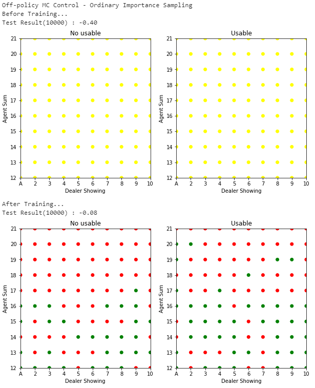
Fig.05 Ordinary Importance Sampling을 사용하는 Off-policy MC Control
500,000번 시뮬레이션 진행한 결과를 이용해 Ordinary Importance Sampling을 사용하는 Off-policy MC Control을 수행한 모습

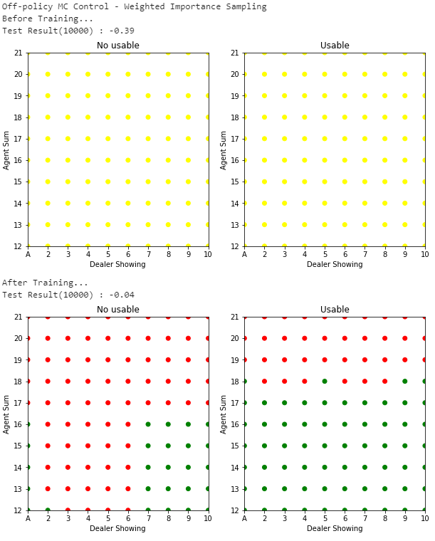
Fig.06 Weighted Importance Sampling을 사용하는 Off-policy MC Control
500,000번 시뮬레이션 진행한 결과를 이용해 Weighted Importance Sampling을 사용하는 Off-policy MC Control을 수행한 모습

Fig.05, Fig.06은 위 코드의 실행 결과를 보여준다. Ordinary Importance Sampling을 사용한 경우(Fig.05), 학습 전에는 보상들의 평균으로 -0.40을 얻다가 학습 후에는 -0.08을 얻는다. Weighted Importance Sampling을 사용한 경우(Fig.06), 학습 전에는 보상들의 평균으로 -0.39을 얻다가 학습 후에는 -0.04을 얻는다.

이 경험이 무작위적인 방법의 역할을 한다. ↩︎
이 경험은 실제가 아닌, 모델(model)에 대한 시뮬레이션 결과여도 된다. 심지어 이 모델은 DP에서 사용하는 완벽한 모델(가능한 모든 전이(transition)를 완벽한 확률 분포로 생성하는 모델)일 필요도 없고, 그저 샘플링(sampling)을 위한 샘플 전이(sample transition)만 생성하는 모델이어도 된다. ↩︎
경험으로부터 얻는 데이터 각각을 샘플(sample)이라 한다. 예를 들어 Episodic Task에선 에피소드 하나가 하나의 샘플이 된다. 그리고 이 샘플로부터 계산한 Return을 Sample Return이라 한다. ↩︎
Continuing Task에 아예 사용하지 못하는 것은 아니나, 일반적이진 않다(거의 사용하지 않는다). ↩︎
이를 episode-by-episode update(= offline update)라 한다. 반댓말은 매 단계(step)마다 업데이트하는, step-by-step update(= online update)이다. ↩︎
First-visit MC Prediction에서 이를 보이는 것은 쉽다: 어떤 행동 $s$ 에 대해, 각 에피소드의 Return들은 $v_{π} (s)$ 에 대한 유한한 분산(variance)을 가지는 iid(independent and identically distributed) 추정값이다. 큰 수의 법칙(law of large numbers)에 의해 이들 추정값들의 평균은 기댓값으로 수렴한다. 각 평균은 그 자체로 편향되지 않은(unbiased) 추정값이고, 오차의 표준편차는 $1 / \sqrt{n}$ 이다(단, $n$ 은 평균된 Return의 개수). 따라서 $n$ 이 커지면 커질수록 오차가 줄어 평균은 $v_{π} (s)$ 으로 수렴하게 된다. Every-visit MC Prediction의 수렴성은 First-visit MC Prediction보다 증명하기 어렵지만 이 역시 수학적으로 반드시 성립한다. ↩︎
즉, 카드카운팅은 의미가 없다. 매 에피소드는 철지히 독립적인 판이다. ↩︎
이렇게 하면 게임 종료 때 받는 보상(terminal reward)이 Return이 된다. ↩︎
에이전트의 의사 결정은 에이전트가 볼 수 있는 정보, 즉 현재 에이전트가 들고 있는 패와, 딜러가 들고 있는 공개된 카드(dealer_showing)를 바탕으로 진행되어야 한다. 이때, 에이전트가 들고 있는 카드들의 점수의 합(agent_sum)이 11점 이하인 경우 무조건 hit을 하면 되므로, agent_sum으로는 12 이상 21 이하의 값만 고려해도 된다. 한편 에이스 카드는 1점 또는 11점으로 계산될 수 있으므로, 에이스 카드를 들고 있는 상황에서 만약 에이스 카드를 11점으로 계산했을 때 bust가 나지 않는다면 무조건 한번 더 hit을 진행할 수 있다. 이렇게 11점으로 계산해도 bust가 나지 않는 에이스 카드를 usable ace라 한다. 에이전트가 들고 있는 패에 usable ace가 있는지 여부도 의사 결정에 영향을 미친다. 따라서, agent_sum, dealer_showing, is_usable, 이 세 가지 변수들에 대해 가능한 모든 조합의 상태만 고려하면 된다. 각각 10가지, 10가지, 2가지 경우의 수가 있으므로, $∥ S ∥ = 200$ 이 된다. ↩︎
모델이 있다면 (비록 실제와 다를 순 있어도) 각 상태에서 어떤 행동을 수행할 수 있는지, 행동의 결과 얼마만큼의 보상이 나오고 어느 상태로 전이하는지 등을 알 수 있다. 이를 이용하면 (DP에서 했던 것처럼) 탐욕적인 선택을 할 수 있다. ↩︎
$π (s) = \underset{a}{\arg \max} q (s, a)$ ↩︎
사실 이 문제는 $v_{π}$ 를 추정할 때도 있을 수 있는 문제긴 하다. 하지만 $v_{π}$ 를 추정할 때의 방문 대상은 각 상태들로, $q_{π}$ 를 추정할 때의 방문 대상인 상태-행동 쌍보다 가짓수가 압도적으로 적다. 그래서 보통 이 문제는 $q_{π}$ 를 추정할 때만 중점적으로 다룬다. ↩︎
그래서 이 문제를 탐색 유지 문제(problem of maintaining exploration)라 한다. ↩︎
말로 풀어 쓰면 다음과 같다 : 현재 상태가 agent_sum = 14, dealer_showing = 10, is_usable = False이고 행동 stick을 선택한 경우, 어떤 상태 $s^{'}$ 으로 가 보상 1을 받을 수 있는 확률은 얼마인가? ↩︎
만약 $v_{π_{k}}$ 가 있다면 모델이 있어야 한다. ↩︎
이 값이 추정의 정도의 상한값이다. ↩︎
그런데 사실 Monte Carlo ES가 항상 최적 정책으로 수렴할 것은 자명해 보이나, 엄밀히 수학적으로 증명되진 않았다고 한다. ↩︎
즉 $π (a ∥ s) = 0$ 이 되는 $(s, a)$ 가 없다는 뜻이다. ↩︎
한 걸음 더 나가 만약 행동 정책 $b$ 가 $ε$ -soft policy이면, 각 상태에서 모든 행동들에 대한 빠짐없는 탐색을 보장할 수 있어 더 좋다. ↩︎
말 그대로 상태와 행동이 번갈아가며 나오는 나열. ex) $A_{1}, S_{2}, A_{2}, S_{3}, A_{3}, \dots, S_{t}$ ↩︎
비록 상태 전이 확률 $p$ 를 모르지만, 분모 분자에 같은 항이 나오므로 모두 약분할 수 있다. ↩︎
예를 들어 $t = 100$ 에 한 에피소드가 끝났다면, 다음 에피소드는 $t = 101$ 에서 시작한다고 하는 것이다. ↩︎
즉 $T (t)$ 는 시간 $t$ 를 포함하는 에피소드의 종료 시점을 의미한다. ↩︎
에피소드 연속적인 시간 단계를 사용했기에 , 두 개의 에피소드에서 각각 $t = 5$ 일 때 상태 $s$ 를 방문했다고 해도 이 두 에피소드를 $J (s)$ 에 구분해서 담을 수 있다. ↩︎
만약 분모가 0이 되면 $V (s) = 0$ 으로 한다. ↩︎
상태 $s$ 를 최초방문하는 에피소드 하나만 보고 First-visit method로 $V (s)$ 를 추정하는 극단적인 상황을 생각해 보자. Weighted Importance Sampling에서는 Importance-sampling ratio $ρ$ 가 약분되어 $V (s) = G_{t}$ 가 된다(아래 첨자는 생략했다). 이때 $G_{t}$ 는 $v_{π} (s)$ 가 아닌 $v_{b} (s)$ 를 나태내는 값이다. 즉 Weighted Importance Sampling은 편향되어 있다(biased). 하지만 Ordinary Importance Sampling에서는 $∥ J (s) ∥ = 1$ 이므로 $V (s) = ρ G_{t}$ 가 된다. 이는 $v_{π} (s)$ 를 나태내는 값이므로 Ordinary Importance Sampling은 편향되어 있지 않다(unbiased). 그러나 에피소드의 수가 많아질수록 편향(bias)는 점점 0으로 수렴하게 된다.
한편 Importance-sampling ratio $ρ$ 는 그 크기의 상한, 하한이 없으므로 값이 매우 클 수 있다. 만약 $ρ = 10$ 이라면(즉, 현재 보고 있는 에피소드의 상태-행동 시퀸스가 행동 정책을 따를 때보다 목표 정책을 따를 때 10배 더 잘 등장한다면) Ordinary Importance Sampling의 추정값은 실제 관측된 Return 값( $G_{t}$ )보다 10배 더 큰 값이 된다. 즉, Ordinary Importance Sampling은 분산이 크다. 비록 현재 보고있는 상태-행동 시퀸스가 목표 정책을 매우 잘 표현하고(representative) 있긴 하지만 말이다. 그러나 Weighted Importance Sampling의 경우 나올 수 있는 값이 최대 1이므로, 분산이 작다. ↩︎
샘플의 수가 많아지면 편향이 작아진다. ↩︎
즉 $W_{n} = ρ_{t_{n} : T (t_{n}) - 1}$ 이 된다. (단, $t_{i}$ 는 $J (s)$ 의 $i$ 번째 원소) ↩︎ ↩︎
단, $C_{0} = 0$ ↩︎

L06. Monte Carlo Methods

MC Method(Monte Carlo Method)란? ​

여담 : k-armed Bandit Problem와의 관련성 ​

MC Prediction(Monte Carlo Prediction) ​

vπ 추정하기 ​

예시 : BlackJack ​

qπ 추정하기 ​

MC Prediction의 장점 ​

MC Control(Monte Carlo Control) ​

MC Policy Iteration(Monte Carlo Policy Iteration) ​

Monte Carlo ES(Monte Carlo with Exploring Starts) ​

구현하기 ​

On-policy MC Control without ES(On-policy Monte Carlo Control without Exploring Starts) ​

구현하기 ​

Off-policy MC Method(Off-policy Monte Carlo Method) ​

Off-policy Prediction ​

Incremental Implementation ​

구현하기 ​

Off-policy MC Control(Off-policy Monte Carlo Control) ​

구현하기 ​

MC Method(Monte Carlo Method)란?

여담 : k-armed Bandit Problem와의 관련성

MC Prediction(Monte Carlo Prediction)

$v_{π}$ 추정하기

예시 : BlackJack

$q_{π}$ 추정하기

MC Prediction의 장점

MC Control(Monte Carlo Control)

MC Policy Iteration(Monte Carlo Policy Iteration)

Monte Carlo ES(Monte Carlo with Exploring Starts)

구현하기

On-policy MC Control without ES(On-policy Monte Carlo Control without Exploring Starts)

구현하기

Off-policy MC Method(Off-policy Monte Carlo Method)

Off-policy Prediction

Incremental Implementation

구현하기

Off-policy MC Control(Off-policy Monte Carlo Control)

구현하기